Delphi Rounds: Consensus and Stability • contentvalidR

Two questions, not one

In a Delphi study, an expert panel rates the same items over several rounds. Between rounds, experts see anonymous feedback on how the panel rated, and they may revise their own ratings. Two different questions come out of that process:

Consensus: do enough experts agree about an item now?
Stability: are experts still changing their ratings?

A panel can agree while still shifting, and it can hold steady without agreeing. Dajani, Sincoff and Talley (1979) argued that a level of agreement is only worth interpreting once responses have stopped changing. delphi_validity() therefore reports the two questions side by side and never folds one into the other.

Decide three things before the first round

Three choices belong in the study protocol, written down before any data arrive, not in the analysis afterwards.

What counts as agreeing. On a 4-point relevance scale this is usually a rating of 3 or 4. In delphi_validity() it is agree_cut.
The consensus threshold. Diamond et al. (2014) reviewed 100 Delphi studies and recommend defining consensus before the study begins. The median threshold in the studies they reviewed was 75%. That figure describes common practice; it is not a validated cut-off. For this reason consensus_threshold has no default. Without one, results are reported descriptively.
How stability will be measured. The default is weighted kappa (below). Cohen (1968) points out that the weights are part of how agreement is defined, and so they must be chosen before the data are collected.

The data

delphi_validity() takes long-format data: one row per expert, item, and round. Here, ten experts rate six statements for relevance on a 1-4 scale over three rounds. Two things happen that are common in real studies. Expert E10 leaves after round 2, and statement S1 reaches consensus in round 2 and is set aside, so nobody rates it in round 3.

round1 <- cbind(
  S1 = c(4, 4, 3, 4, 3, 4, 2, 4, 3, 4),
  S2 = c(3, 4, 3, 2, 4, 3, 4, 3, 2, 4),
  S3 = c(2, 1, 2, 2, 1, 3, 2, 1, 2, 2),
  S4 = c(4, 2, 3, 1, 4, 2, 3, 1, 4, 2),
  S5 = c(2, 3, 2, 3, 2, 4, 3, 2, 3, 2),
  S6 = c(3, 2, 4, 1, 3, 2, 4, 1, 3, 2)
)
round2 <- cbind(
  S1 = c(4, 4, 4, 4, 3, 4, 3, 4, 3, 4),
  S2 = c(4, 4, 4, 4, 4, 4, 4, 3, 4, 4),
  S3 = c(2, 1, 2, 2, 1, 2, 2, 1, 2, 2),
  S4 = c(4, 2, 3, 1, 4, 1, 3, 2, 4, 2),
  S5 = c(3, 3, 2, 3, 3, 4, 3, 2, 3, 3),
  S6 = c(2, 3, 1, 4, 2, 3, 1, 4, 2, 3)
)
round3 <- cbind(  # E10 has left; S1 was set aside
  S2 = c(4, 4, 4, 4, 4, 4, 4, 4, 4),
  S3 = c(2, 1, 2, 2, 1, 2, 2, 1, 2),
  S4 = c(4, 1, 3, 1, 4, 1, 3, 2, 4),
  S5 = c(3, 3, 3, 3, 3, 4, 3, 3, 3),
  S6 = c(3, 2, 4, 1, 3, 2, 4, 1, 3)
)

to_long <- function(m, round) {
  data.frame(expert = paste0("E", seq_len(nrow(m))),
             item = rep(colnames(m), each = nrow(m)),
             round = round, rating = as.vector(m))
}
ratings <- rbind(to_long(round1, 1), to_long(round2, 2), to_long(round3, 3))
head(ratings)
#>   expert item round rating
#> 1     E1   S1     1      4
#> 2     E2   S1     1      4
#> 3     E3   S1     1      3
#> 4     E4   S1     1      4
#> 5     E5   S1     1      3
#> 6     E6   S1     1      4

If your data are already long, name the columns with expert_col, item_col, round_col, and rating_col.

Fitting the workflow

The threshold of 75% was fixed in this example’s protocol before the study. The seed makes the bootstrap intervals reproducible.

fit <- delphi_validity(ratings, lo = 1, hi = 4, consensus_threshold = 0.75,
                       seed = 2026)
fit
#> contentvalidR Delphi analysis
#> -----------------------------
#> Items: 6 | Experts: 10 | Rounds: 3 (1, 2, 3)
#> Experts per round: 10, 10, 9
#> Agreement: a rating of 3 or higher on the 1-4 scale. Consensus threshold:
#> 75%, fixed before the study.
#> Stability: weighted kappa (quadratic weights) between consecutive rounds
#> 
#> 3 of 6 items reached consensus in their last round.
#> No consensus: S3, S4, S6
#> 
#> Item-level evidence (last round, and the last pair of rounds)
#>  item     decision last round  n agree unchanged kappa        95% CI
#>    S1    Consensus          2 10  1.00       .80   .71   [.20, 1.00]
#>    S2    Consensus          3  9  1.00       .89   .00            NA
#>    S3 No consensus          3  9   .00      1.00  1.00  [1.00, 1.00]
#>    S4 No consensus          3  9   .56       .89   .96   [.84, 1.00]
#>    S5    Consensus          3  9  1.00       .78   .53   [.00, 1.00]
#>    S6 No consensus          3  9   .56       .00  -.99 [-1.00, -.30]
#> 
#> agree: share of experts agreeing in the item's last round. unchanged: share
#> who kept their rating between the last two rounds.
#> 
#> Stability trend (kappa) by pair of rounds
#>  item  1->2 2->3
#>    S1   .71   NA
#>    S2   .04  .00
#>    S3   .83 1.00
#>    S4   .92  .96
#>    S5   .63  .53
#>    S6 -1.00 -.99
#> 
#> Share of experts who kept their rating, by pair of rounds
#>  item 1->2 2->3
#>    S1  .80   NA
#>    S2  .50  .89
#>    S3  .90 1.00
#>    S4  .80  .89
#>    S5  .70  .78
#>    S6  .00  .00
#> 
#> Notes
#>   S2 (2->3): Every expert gave the same rating in one of the two rounds, so
#>     kappa is 0 however many kept their rating. Read the share who kept their
#>     rating instead.
#> 
#> In some resamples kappa was undefined because every resampled rating fell in
#> one category. Those intervals use the remaining resamples (n_boot_usable in
#> details$stability), so treat them as rough.
#> 
#> Read kappa as a trend across rounds, beside the share of experts who kept
#> their rating (unchanged), not against a cut-off: kappa falls as a panel
#> converges on one category, so a stable panel can show a low kappa (Holey et
#> al., 2007).
#> 
#> The kappa intervals resample the experts (Klar et al., 2002). With fewer than
#> about 40 experts they cover less than their stated 95%, so read them as rough
#> indications of precision, not as tests.
#> 
#> The panel changed size across rounds (10, 10, 9 experts). Stability uses only
#> the experts who rated an item in both rounds, and a result from fewer experts
#> is weaker evidence.
#> 
#> How the stability statistic works
#>   Stability is weighted kappa between each expert's ratings in consecutive
#>   rounds (Holey et al., 2007), with quadratic weights. A change of two scale
#>   points counts four times a change of one. With these weights kappa equals
#>   the intraclass correlation of the two rounds' ratings, so a shift of the
#>   whole panel counts as instability (Fleiss & Cohen, 1973). No verbal labels
#>   such as 'substantial' are shown, because kappa falls when ratings converge,
#>   which is what a Delphi aims for: Holey et al. saw a low kappa for their
#>   most-agreed statement.
#> 
#>   The intervals are percentile bootstraps that resample the experts, the
#>   units the two rounds cross-classify: the procedure Klar et al. (2002)
#>   describe for kappa. They evaluated it for an unweighted kappa on two
#>   categories, and a nominal 95% interval covered about 83% of the time with
#>   20 units and 91% with 30, reaching 94% only from 40 up.
#> 
#> What these columns mean
#>   agree -- Share of experts agreeing. Share of experts at or above the
#>       agreement cut in a round; consensus means reaching the preset
#>       threshold.
#>   unchanged -- Share of experts keeping their rating. Share of experts
#>       giving the same rating in two consecutive rounds (1 means nobody
#>       changed).
#>   kappa -- Weighted kappa between rounds. Chance-corrected agreement of
#>       each expert's ratings across two rounds; read it as a trend, not
#>       against a cut-off.
#> 
#> What the decisions mean
#>   Consensus -- reached the consensus threshold in its last round.
#>   No consensus -- did not reach the consensus threshold.
#> 
#> Full definitions: contentvalid_glossary(). To hide this key:
#> options(contentvalidR.show_key = FALSE).
#> 
#> Consensus is not correctness, and 'No consensus' is not an instruction to
#> drop an item. Read these results with the experts' comments.

The printout ends with a key: how the stability statistic works, and what each column and decision means. The two caveats above the key print either way. The rest of this article turns the key off, to keep the output short:

options(contentvalidR.show_key = FALSE)

Reading consensus

The agree column (prop_agree in fit$results) is the share of experts who rated the item at or above agree_cut in its last round. On a relevance scale this is the item’s I-CVI. Three statements (S1, S2, and S5) reached the 75% threshold. S1’s last round is round 2, because it was set aside once it reached consensus.

Look at S3. Nobody rated it relevant, which looks like “no consensus”. But the panel does agree: every expert rated it below the cut. The interpretation says so. Whether agreement in that direction counts as consensus to exclude an item is for your protocol to define, not for the software to decide.

shown <- fit$results[fit$results$item %in% c("S3", "S4"), ]
writeLines(strwrap(paste0(shown$item, ": ", shown$interpretation),
                   width = 72, exdent = 4))
#> S3: No consensus in the last round: 0% agreed, against a threshold of
#>     75%. The panel did agree in the other direction: 100% rated it
#>     below the agreement cut. Whether that is consensus to exclude is
#>     for your protocol to say.
#> S4: No consensus in the last round: 56% agreed, against a threshold of
#>     75%. Consider another round, rewording, or reporting the item as
#>     without consensus.

Reading stability

Read the unchanged column (prop_unchanged in fit$results) first. It is the plainest measure: the share of experts who gave exactly the same rating again. Then read the kappa trend beside it. Kappa is weighted kappa between each expert’s ratings in two consecutive rounds (Holey et al., 2007). With the default quadratic weights, it equals the intraclass correlation of the two rounds’ ratings (Fleiss & Cohen, 1973). A shift of the whole panel after feedback therefore counts as instability.

The six statements show the main patterns:

S3 and S4 are stable. Almost every expert kept their rating, and kappa is high: between .83 and 1 in every pair of rounds. But S4 is stable without consensus: the panel is split (56% agreeing) and staying split. Another round is unlikely to change that. Dajani et al. (1979) treat a stable split as a result in its own right, to be reworded or reported rather than iterated away.
S2 converged to unanimity. In round 3 every expert rated it 4. Of the experts who rated it in both rounds, 89% kept their rating, yet kappa is 0. When every rating in a round is the same, there is no room left above chance, so kappa is 0 no matter how many experts held steady. The output flags this and points you to the share who kept their rating.
S5 formed consensus while kappa fell, from .63 to .53. As ratings bunch near 3, kappa has less room to show agreement. This is the same pattern Holey et al. (2007) reported: their most-agreed statement had their lowest kappa. With nine or ten experts, the intervals run from about 0 to 1.
S6 is unstable. No expert kept their rating, and kappa is negative because experts swapped positions.

These patterns are why the output gives kappa no verbal labels such as “moderate” or “substantial”. Landis and Koch (1977), who introduced those labels, called their divisions clearly arbitrary. And a label would tend to get worse as a Delphi succeeds, because convergence lowers kappa. Read kappa as a trend, next to the unchanged column.

The full table, with every pair of rounds, is in details$stability:

st <- fit$details$stability
cols <- c("prop_unchanged", "value", "lower", "upper")
st[cols] <- round(st[cols], 2)
st[c("item", "from_round", "to_round", "n_paired", cols)]
#>    item from_round to_round n_paired prop_unchanged value lower upper
#> 1    S1          1        2       10           0.80  0.71  0.20  1.00
#> 2    S2          1        2       10           0.50  0.04 -0.04  0.40
#> 3    S2          2        3        9           0.89  0.00    NA    NA
#> 4    S3          1        2       10           0.90  0.83  0.44  1.00
#> 5    S3          2        3        9           1.00  1.00  1.00  1.00
#> 6    S4          1        2       10           0.80  0.92  0.73  1.00
#> 7    S4          2        3        9           0.89  0.96  0.84  1.00
#> 8    S5          1        2       10           0.70  0.63  0.00  1.00
#> 9    S5          2        3        9           0.78  0.53  0.00  1.00
#> 10   S6          1        2       10           0.00 -1.00 -1.00 -0.36
#> 11   S6          2        3        9           0.00 -0.99 -1.00 -0.30

n_paired counts the experts who rated the item in both rounds. It drops to 9 in the second pair because E10 left.

Seeing the trends

Both questions are trends across rounds, which a plot reads better than a table of round pairs:

plot(fit)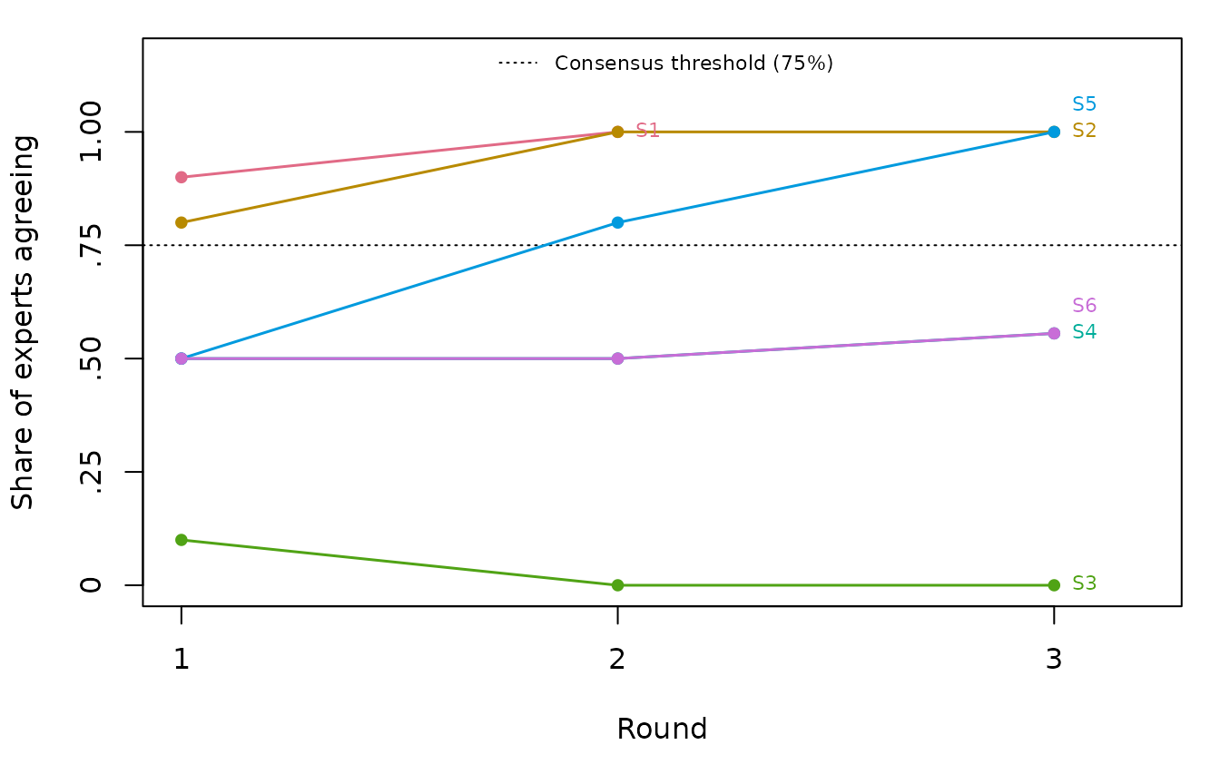

Share of experts agreeing with each statement, by round, with a dotted line at the 75% consensus threshold.

S1’s line stops at round 2, because that is where it settled and was set aside. The dotted line is the threshold you fixed in advance; with no threshold set, no line is drawn, because the analysis applies none.

plot(fit, which = "stability")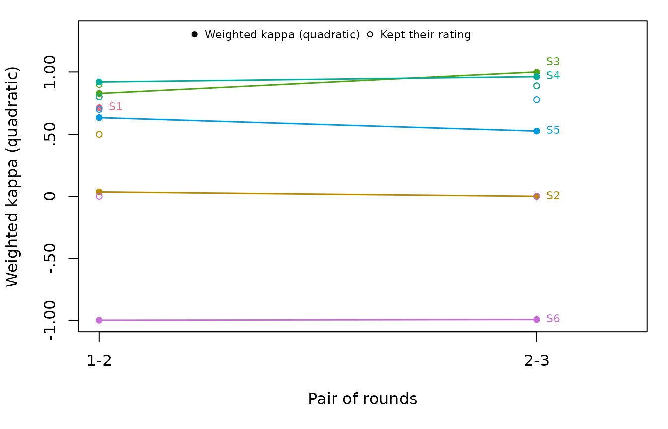

Weighted kappa for each statement across pairs of rounds, with open circles showing the share of experts who kept their rating.

Filled points are kappa, open circles the share of experts who kept their rating. S6 sits at the bottom on both, and S2’s kappa of 0 sits well below its share unchanged, which is the unanimous-round case described above. There are no shaded “good” and “poor” bands behind kappa, for the same reason there are no verbal labels.

Both plots summarize. The distribution view shows every rating, one bar per round for each statement, split at the agreement cut (Heiberger & Robbins, 2014). The right-hand length is the share agreeing, read against the dashed consensus threshold:

plot(fit, which = "distribution")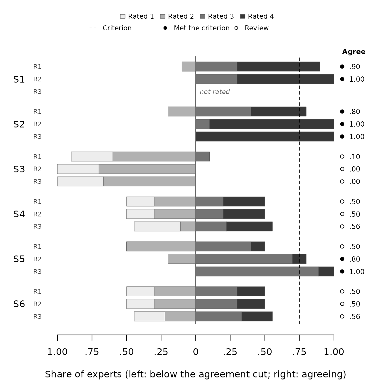

Rating distributions for six statements over three rounds, one bar per round, split at the agreement cut of 3, with a dashed line at the 75% consensus threshold. S1 is not rated in round 3, having reached consensus in round 2; S2 moves to unanimous 4s by round 3; nearly every expert rates S3 below the cut in every round.

S2’s bars show a panel converging, and S3’s a panel agreeing that the statement does not belong: agreement in the other direction, which the printout notes in words and the bars show at a glance. Add apa = FALSE for a color version for slides or a poster.

Why the default looks at individual experts

S6 is the reason stability is measured expert by expert. Under the 15% rule of Scheibe et al. (1975/2002), which compares the two rounds’ overall rating distributions, S6 looks perfectly stable:

pc <- delphi_validity(ratings, lo = 1, hi = 4, consensus_threshold = 0.75,
                      stability = "percent_change")
s6 <- pc$details$stability[pc$details$stability$item == "S6", ]
s6$value <- round(s6$value, 2)
s6[c("item", "from_round", "to_round", "prop_unchanged", "value", "stable")]
#>    item from_round to_round prop_unchanged value stable
#> 10   S6          1        2              0  0.00   TRUE
#> 11   S6          2        3              0  0.11   TRUE

The distribution barely moved: the net change is 0% and then 11%. Yet no expert kept their rating. Experts traded places, so the totals stayed the same. Chaffin and Talley (1980) made exactly this point against group-level stability tests. Every published method remains available through stability, and each one prints its own limits:

`stability`	What it measures	Reads as stable when	Main limitation
`"kappa"` (default)	Each expert’s agreement with their own earlier rating, corrected for chance	Read as a trend; no cut-off	Falls as ratings converge
`"lambda"`	How well an earlier rating predicts the later one	Read as a trend	Predictability, not agreement; undefined if the later round is unanimous
`"chisq_individual"`	Whether later ratings depend on earlier ones	p < alpha	Association, not agreement; needs expected counts of 5 or more
`"chisq_group"`	Whether the two rounds’ distributions differ	p >= alpha	Small panels look stable by default; misses experts swapping answers
`"percent_change"`	Net movement of the distribution	Change below 15%	No statistical basis; misses swapping; coarse with small panels

The two chi-square tests read in opposite directions: one counts a significant result as stable, the other a non-significant one. The printout always says which is which.

Relevance evidence round by round

Each round is also analyzed with expert_validity(), so the usual relevance evidence (I-CVI, Aiken’s V, and their intervals) is available round by round. compare_rounds() reads those fits directly:

do.call(compare_rounds, unname(fit$details$round_fits))
#> contentvalidR comparison across pretest rounds
#> ----------------------------------------------
#> Workflow: expert-panel | Rounds: 3 | Units compared: 6
#> 
#> Status by round
#>  item   Round 1   Round 2   Round 3       change
#>    S1 Supported Supported      <NA>      Removed
#>    S2 Supported Supported Supported    Unchanged
#>    S3    Review    Review    Review    Unchanged
#>    S4    Review    Review    Review    Unchanged
#>    S5    Review Supported Supported Strengthened
#>    S6    Review    Review    Review    Unchanged
#> 
#> Round-to-round summary
#>     from      to compared unchanged stronger weaker added removed same settings
#>  Round 1 Round 2        6         5        1      0     0       0           yes
#>  Round 2 Round 3        5         5        0      0     0       1           yes
#> 
#> Settings were identical across rounds, so these transitions can be read as
#> changes in evidence.
#> 
#> A status change means the evidence crossed a criterion, not that an item
#> improved by a measurable amount. An item sitting near a boundary can move on
#> a very small change. Read transitions alongside each round's index values.

S1 shows as Removed in round 3 because it was set aside after reaching consensus. S5 strengthened once experts converged.

Reporting

content_report() gives a compact table for a manuscript:

content_report(fit)
#>  item last round experts agree unchanged stability        95% CI     decision
#>    S1          2      10  1.00       .80       .71   [.20, 1.00]    Consensus
#>    S2          3       9  1.00       .89       .00            NA    Consensus
#>    S3          3       9   .00      1.00      1.00  [1.00, 1.00] No consensus
#>    S4          3       9   .56       .89       .96   [.84, 1.00] No consensus
#>    S5          3       9  1.00       .78       .53   [.00, 1.00]    Consensus
#>    S6          3       9   .56       .00      -.99 [-1.00, -.30] No consensus

Diamond et al. (2014) recommend that a Delphi report state the definition of consensus and its threshold (decided before the study), the criteria for stopping, and the criteria for dropping items. Also report:

the number of rounds and experts in each round;
the stability statistic, and the weights if it is kappa;
the number of bootstrap resamples and the seed.

Carrying a Delphi forward

When the panel is finished, content_handoff() packages the items that survived, with the evidence behind each decision, for the empirical stage:

handoff <- content_handoff(fit, keep = "Supported")
handoff$item_evidence[c("item", "carried", "status", "n_judges", "round")]
#>   item carried    status n_judges round
#> 1   S1    TRUE Supported       10     2
#> 2   S2    TRUE Supported        9     3
#> 3   S3   FALSE    Review        9     3
#> 4   S4   FALSE    Review        9     3
#> 5   S5    TRUE Supported        9     3
#> 6   S6   FALSE    Review        9     3

round is the round each item settled in, so S1 carries round 2: it reached consensus there and was set aside. Every other workflow writes one constant into that column, because one fit is one round.

Each item’s relevance evidence comes from its own last round, with intervals, and the stability evidence travels beside it:

st <- handoff$item_statistics
unique(st$statistic)
#> [1] "I-CVI"                      "Aiken's V"                 
#> [3] "modified kappa"             "proportion unchanged"      
#> [5] "weighted kappa (quadratic)"

Stability is carried as evidence, not as a reason to keep or drop an item, just as it does not set an item’s status above. See vignette("handoff-to-empirical-validation") for what the object holds and how a downstream package reads it.

What this analysis does not establish

Consensus is agreement among these experts. It is not, by itself, evidence that an item is valid. Feedback between rounds can also press experts toward agreement they do not hold: Scheibe et al. (1975/2002) observed that participants who conformed most strongly were the least satisfied with the process. A No consensus result is not an instruction to drop an item, and Consensus is not an instruction to keep one. Read these results together with the experts’ comments, the construct definition, and the rest of the content-validity evidence.

References

Chaffin, W. W., & Talley, W. K. (1980). Individual stability in Delphi studies. Technological Forecasting and Social Change, 16(1), 67–73. https://doi.org/10.1016/0040-1625(80)90074-8

Cohen, J. (1968). Weighted kappa: Nominal scale agreement provision for scaled disagreement or partial credit. Psychological Bulletin, 70(4), 213–220. https://doi.org/10.1037/h0026256

Dajani, J. S., Sincoff, M. Z., & Talley, W. K. (1979). Stability and agreement criteria for the termination of Delphi studies. Technological Forecasting and Social Change, 13(1), 83–90. https://doi.org/10.1016/0040-1625(79)90007-6

Diamond, I. R., Grant, R. C., Feldman, B. M., Pencharz, P. B., Ling, S. C., Moore, A. M., & Wales, P. W. (2014). Defining consensus: A systematic review recommends methodologic criteria for reporting of Delphi studies. Journal of Clinical Epidemiology, 67(4), 401–409. https://doi.org/10.1016/j.jclinepi.2013.12.002

Fleiss, J. L., & Cohen, J. (1973). The equivalence of weighted kappa and the intraclass correlation coefficient as measures of reliability. Educational and Psychological Measurement, 33(3), 613–619. https://doi.org/10.1177/001316447303300309

Heiberger, R. M., & Robbins, N. B. (2014). Design of diverging stacked bar charts for Likert scales and other applications. Journal of Statistical Software, 57(5), 1–32. https://doi.org/10.18637/jss.v057.i05

Holey, E. A., Feeley, J. L., Dixon, J., & Whittaker, V. J. (2007). An exploration of the use of simple statistics to measure consensus and stability in Delphi studies. BMC Medical Research Methodology, 7, 52. https://doi.org/10.1186/1471-2288-7-52

Landis, J. R., & Koch, G. G. (1977). The measurement of observer agreement for categorical data. Biometrics, 33(1), 159–174. https://doi.org/10.2307/2529310

Scheibe, M., Skutsch, M., & Schofer, J. (2002). Experiments in Delphi methodology. In H. A. Linstone & M. Turoff (Eds.), The Delphi method: Techniques and applications (pp. 257–281). https://www.foresight.pl/assets/downloads/publications/Turoff_Linstone.pdf (Original work published 1975)