From item audit to exploratory structure • nomologR

Why this workflow is staged

Exploratory factor analysis is not a scale-purification button. Before interpreting an exploratory factor solution, researchers should know what items are being analyzed, how they are coded, whether the correlation model matches the intended measurement level, and how many dimensions are substantively plausible.

nomologR therefore separates three questions:

nomo_screen() — What does the item and response data look like?
nomo_factors() — How many latent dimensions deserve investigation?
nomo_efa() — What does a requested exploratory structure look like?

The handoff is deliberate: no stage silently deletes items, changes the requested factor count, or treats a numerical reference value as proof.

A teaching dataset with a known answer

nomo_demo_continuous was simulated from a documented population model, so the package’s evidence can be checked against the truth:

two factors, A and B, correlated .40;
items a1–a4 and b1–b4 are ordinary indicators (population loadings .70 to .80);
a5 cross-loads on both factors (.45 on A and .35 on B);
b5 is a weak indicator (.30 on B);
a2 and b3 contain a small amount of missing data.

str(nomo_demo_continuous)
#> 'data.frame':    500 obs. of  10 variables:
#>  $ a1: num  2.23 3.47 4.8 2.87 5.22 4.02 3.23 3.12 3.62 4.66 ...
#>  $ a2: num  1.46 3.06 4.16 2.46 3.71 6.06 4.16 3.45 NA 5.27 ...
#>  $ a3: num  2.25 4.71 4.08 3.45 5.94 4.3 3.39 3.41 3.21 5.31 ...
#>  $ a4: num  2.59 3.39 4.59 3.85 4.01 3.65 4.09 3.81 4.77 5.16 ...
#>  $ a5: num  1.85 3.23 4.54 4.22 3.62 4.67 4.14 3.46 4.95 3.08 ...
#>  $ b1: num  2.67 4.05 5.31 4.6 3.57 3.11 4.16 3.99 3.49 2.71 ...
#>  $ b2: num  4.21 3.91 3.65 3.72 3.94 3.01 4.32 2.72 3.17 3.95 ...
#>  $ b3: num  2.33 4.72 4.85 4.63 2.84 2.95 3.75 4.02 3.69 3.08 ...
#>  $ b4: num  4.79 3.72 4.24 4.27 4.6 2.28 5.01 4.62 2.94 2.87 ...
#>  $ b5: num  3.42 4.47 5.4 4.38 3.87 2.97 4.75 5.63 3.65 2.97 ...
colSums(is.na(nomo_demo_continuous))
#> a1 a2 a3 a4 a5 b1 b2 b3 b4 b5 
#>  0 15  0  0  0  0  0 12  0  0

With real data, of course, nobody hands you the population model. The point of a known-answer dataset is to learn what the evidence looks like when you do know what is true.

Step 1: audit the items

scr <- nomo_screen(nomo_demo_continuous)
summary(scr)
#> <nomo_screen summary> Item and data audit
#> Cases: 500 | Items: 10 | Flags: 1 review, 0 concern
#> Items with missing responses: 2 | Constant: 0 | All missing: 0
#> Relationship eligible: 10
#> 
#> Item review
#>   Item  Type        Missing  Top share  Item-rest r  Flag
#>   a1    continuous     0.0%       1.0%        0.559
#>   a2    continuous     3.0%       1.2%        0.580
#>   a3    continuous     0.0%       1.0%        0.511
#>   a4    continuous     0.0%       1.2%        0.549
#>   a5    continuous     0.0%       1.6%        0.588
#>   b1    continuous     0.0%       1.6%        0.602
#>   b2    continuous     0.0%       1.4%        0.513
#>   b3    continuous     2.4%       1.0%        0.571
#>   b4    continuous     0.0%       1.2%        0.481
#>   b5    continuous     0.0%       1.4%        0.279  review
#>   Top share is the proportion of responses in the most common category.
#> 
#> Flagged items
#>   - b5 (review): `b5` has a corrected item-rest correlation of r = 0.28 (n =
#>     473), below the teaching reference.
#> 
#> Flags are review aids, not decisions to keep or delete an item.

The screening object is descriptive and diagnostic. The missing values in a2 and b3 are visible here, before any model decides how to handle them. A flag is a reason to inspect an item or a coding decision, not an instruction to remove it.

plot(scr)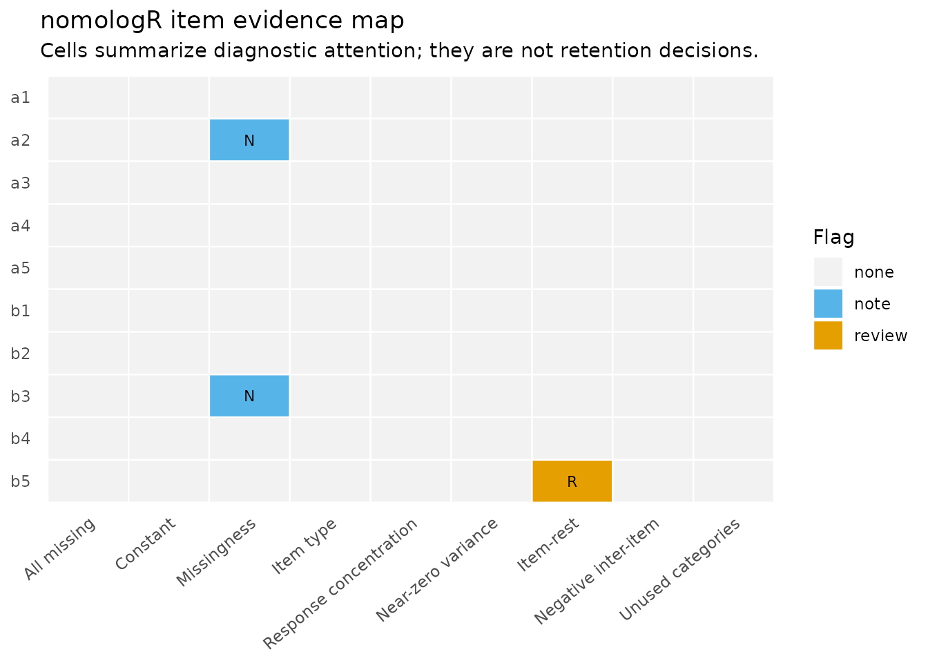

Careless responding

The audit above is about items. A second question is about respondents: did everyone read the items? The data below is simulated: four five-point scales of six items, two reverse keyed in each, with 15 respondents who gave the same answer throughout and 15 who answered at random.

set.seed(34)
n <- 400
factors <- replicate(4, rnorm(n))
respond <- function(f) pmin(5, pmax(1, round(3 + f + rnorm(n, sd = .7))))

responses <- list()
reverse <- character()
scales <- list()
for (s in 1:4) {
  items <- paste0("s", s, "_", 1:6)
  for (j in 1:6) {
    r <- respond(factors[, s])
    if (j %in% c(2, 5)) {
      r <- 6 - r
      reverse <- c(reverse, items[j])
    }
    responses[[items[j]]] <- r
  }
  scales[[paste0("S", s)]] <- items
}
survey <- as.data.frame(responses)
survey[1:15, ] <- 3
survey[16:30, ] <- matrix(sample(1:5, 15 * ncol(survey), TRUE), 15, ncol(survey))

effort = TRUE adds case-level indices from the careless-responding literature. Reverse keying and the response range are declared rather than inferred, because a range guessed from the data is wrong whenever a category went unused:

careful <- nomo_screen(
  survey,
  effort = TRUE,
  scales = scales,
  reverse = reverse,
  scale_range = c(1, 5)
)
careful
#> <nomo_screen> Item and data audit
#> Cases: 400 | Candidate items: 24
#> Items with missing responses: 0 | Constant: 0 | All missing: 0
#> Relationship diagnostics: 24 eligible items | 24 item-rest estimates
#> Response concentration flags: 0 | Near-zero variance: 0
#> Careless-responding flags: 75 cases | long-string 15 | antonym 27 | synonym 36
#>   Cases are flagged, never removed. Indices disagree by design; see the
#>   decision log.
#> Decision log: 27 info, 16 review, 0 concern
#> No rows or items were removed or modified.

The indices do not agree, and they are not supposed to. Compare what two of them say about the respondents who answered identically throughout:

nomo_table(careful, "effort")[1:3, c(
  "row", "long_string", "inter_item_sd", "flagged_by"
)]
#> # A tibble: 3 × 4
#>     row long_string inter_item_sd flagged_by 
#>   <int>       <dbl>         <dbl> <chr>      
#> 1     1          24             0 long_string
#> 2     2          24             0 long_string
#> 3     3          24             0 long_string

Long-string flags every one of them. Inter-item standard deviation gives them a score of zero, the most consistent possible. That is not a contradiction. Inter-item standard deviation detects random responding (Marjanovic et al., 2015), and a respondent who never varies is not random. Sorting on it alone would keep exactly the respondents long-string exists to find, which is why Curran (2016) recommends using these methods in series.

Two further cautions come from the sources. Huang et al. (2012) found the indices they recommended identified attentive respondents well and random responders poorly, so a case with no flag has not been shown to be attentive. And each antonym, synonym, and even-odd value is a correlation computed across a handful of pairs or scales; with few of them, attentive respondents cross zero by chance, and the decision log says so.

Nothing is removed. Deciding what to do with a flagged respondent is a research decision, made with the design and the data collection in view.

Step 2: investigate factor retention

fac <- nomo_factors(
  nomo_demo_continuous,
  criterion_set = "core",
  seed = 2026
)
summary(fac)
#> <nomo_factors summary> Factor-retention evidence
#> Cases: 500 | Items: 10 | Correlation: pearson | Criteria: core
#> 
#> Retention evidence
#>   Method              Factors  Role
#>   Parallel analysis         2  primary
#>   MAP (original TR2)        2  complementary
#>   MAP (revised TR4)         2  complementary
#> 
#> Parallel-analysis rule sensitivity
#>   Rule        Factors  Used
#>   percentile        2  selected
#>   mean              2
#>   crawford          2
#> 
#> Criteria requested but not run
#>   - Empirical Kaiser criterion: EKC needs one common sample size for the
#>     analyzed matrix; pairwise missing-data handling produced varying pairwise
#>     Ns.
#> 
#> Concordance across criterion families
#>   Factors  Families  Which
#>         2         2  Parallel analysis; MAP
#> 
#> Supporting adequacy evidence
#>   - KMO: 0.874
#>   - Bartlett: Bartlett's test was not computed because pairwise missing-data
#>     handling does not provide one common sample size for the full matrix.
#> 
#> Synthesis
#>   All 2 available criterion families (3 methods) point to 2 factors. Related
#>   methods within a family are grouped before concordance is summarized; this
#>   is strong converging evidence for investigating that solution, not proof of
#>   dimensionality. 1 requested method was not evaluated; see criterion status
#>   for the documented reason.
#> 
#> Factor counts are candidates for investigation, not automatic dimensionality
#> verdicts. Common-factor eigenvalues come from a reduced common-variance
#> matrix; later values can be negative.

Parallel analysis is the primary retention evidence, with MAP and the empirical Kaiser criterion (EKC) providing complementary evidence. Here parallel analysis and both MAP variants agree on two dimensions, which matches the population model. When methods disagree, the disagreement is part of the result rather than something nomologR resolves with a majority vote.

Notice that EKC was requested but not run. The default pairwise-complete correlations use different numbers of cases for different item pairs (because of the missing values in a2 and b3), and EKC needs one common sample size. nomologR reports that reason instead of silently substituting another criterion. Choosing missing = "complete" would make EKC available, at the cost of analyzing only the cases with no missing items — a trade-off for the researcher to make and record.

plot(fac, type = "scree")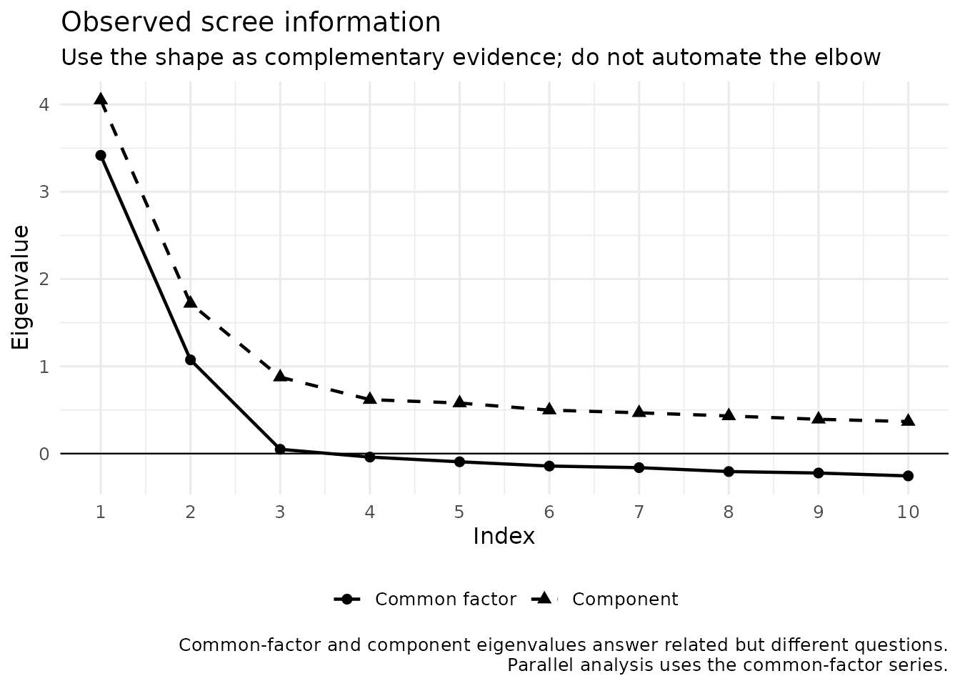

Historical note: eigenvalues greater than one

For decades, many researchers retained every component with an eigenvalue greater than one (Guttman, 1954; Kaiser, 1960), often as part of the “Little Jiffy” routine of principal components, eigenvalues greater than one, and varimax rotation. Simulation research has shown that this rule frequently retains too many dimensions, and parallel analysis (Horn, 1965) is now preferred. nomologR can display the legacy rule with criterion_set = "all", labeled as historical context and excluded from the synthesis, so that learners can recognize it in published work without relying on it.

Step 3: hand the retention evidence into EFA

efa <- nomo_efa(
  nomo_demo_continuous,
  factors = fac
)
summary(efa)
#> <nomo_efa summary> Exploratory factor analysis
#> Cases: 500 | Items: 10 | Factors: 2 (from nomo_factors())
#> Correlation: pearson | Extraction: minres | Rotation: oblimin
#> Supporting adequacy: KMO 0.874
#> 
#> Item structure
#>   Item  Factor  Loading  Next factor  Loading  Communality  Flag
#>   a1    F1        0.808  F2            -0.044        0.624
#>   a2    F1        0.709  F2             0.064        0.547
#>   a3    F1        0.667  F2             0.015        0.454
#>   a4    F1        0.770  F2            -0.038        0.569
#>   a5    F1        0.414  F2             0.335        0.406  review
#>   b1    F2        0.783  F1             0.014        0.623
#>   b2    F2        0.693  F1            -0.020        0.469
#>   b3    F2        0.783  F1            -0.007        0.608
#>   b4    F2        0.637  F1            -0.012        0.400  review
#>   b5    F2        0.332  F1             0.029        0.120  concern
#> 
#> Flagged items
#>   - a5 (review): secondary loading |0.34| meets/exceeds the 0.30 cross-loading
#>     reference
#>   - b4 (review): communality 0.40 is below the 0.40 teaching reference
#>   - b5 (concern): primary loading |0.33| is below the 0.40 teaching reference;
#>     communality 0.12 is below the 0.40 teaching reference
#> 
#> Factor correlations
#>   Factor 1  Factor 2      r
#>   F1        F2        0.439
#> 
#> Largest residual correlations
#>   Off-diagonal RMSR: 0.018
#>   Item 1  Item 2  Residual
#>   b4      b5         0.042
#>   a5      b5        -0.039
#>   a4      b5         0.038
#>   a2      a5         0.030
#>   b2      b5        -0.028
#> 
#> Numerical references trigger inspection, not automatic deletion or hidden
#> refitting.

Passing the nomo_factors object carries forward the item set, modeling types, correlation model, and missing-data strategy. The primary parallel-analysis count becomes the requested EFA factor count. If the retention evidence had identified neighboring plausible solutions, nomo_efa() would record that context and recommend comparing them rather than treating the handoff as proof.

Read the item table as evidence, not a deletion list

item_view <- efa$item_summary[, c(
  "item", "primary_factor", "primary_loading", "secondary_loading",
  "communality", "attention"
)]
item_view
#> # A tibble: 10 × 6
#>    item  primary_factor primary_loading secondary_loading communality attention 
#>    <chr> <chr>                    <dbl>             <dbl>       <dbl> <chr>     
#>  1 a1    F1                       0.808          -0.0444        0.624 KEEP      
#>  2 a2    F1                       0.709           0.0643        0.547 KEEP      
#>  3 a3    F1                       0.667           0.0153        0.454 KEEP      
#>  4 a4    F1                       0.770          -0.0377        0.569 KEEP      
#>  5 a5    F1                       0.414           0.335         0.406 REVIEW    
#>  6 b1    F2                       0.783           0.0141        0.623 KEEP      
#>  7 b2    F2                       0.693          -0.0200        0.469 KEEP      
#>  8 b3    F2                       0.783          -0.00673       0.608 KEEP      
#>  9 b4    F2                       0.637          -0.0119        0.400 REVIEW    
#> 10 b5    F2                       0.332           0.0286        0.120 STRONG RE…

Compare the table with the known population model:

a5 receives REVIEW. Its secondary loading of 0.34 reaches the cross-loading reference, exactly the feature built into the data.
b5 receives STRONG REVIEW. Its primary loading of 0.33 and communality of 0.12 reflect the weak population loading.
b4 receives REVIEW even though its population loading is .70. Its sample communality of 0.400 sits essentially at the .40 reference. This is sampling variability around a teaching reference — a reminder that references are prompts, not cliffs.

KEEP means that no configured numerical teaching reference fired. It does not mean that theory, wording, content coverage, redundancy, or external validity evidence has approved the item. Likewise, REVIEW does not mean “delete.” Defensible options for a5 include retaining it because its content is essential, revising its wording, or evaluating a model without it — and recording the rationale either way.

These are the values in the returned table. print() and summary() show the same flags in the package’s display wording: no flag for KEEP, “review” for REVIEW, and “concern” for STRONG REVIEW.

Pattern versus structure matrices

With oblique rotation, the pattern matrix contains regression-like factor coefficients and is the primary matrix for interpreting which indicators define which factors. The structure matrix contains item–factor correlations and also reflects the correlation between factors.

round(efa$pattern_matrix, 2)
#>       F1    F2
#> a1  0.81 -0.04
#> a2  0.71  0.06
#> a3  0.67  0.02
#> a4  0.77 -0.04
#> a5  0.41  0.34
#> b1  0.01  0.78
#> b2 -0.02  0.69
#> b3 -0.01  0.78
#> b4 -0.01  0.64
#> b5  0.03  0.33
round(efa$structure_matrix, 2)
#>      F1   F2
#> a1 0.79 0.31
#> a2 0.74 0.38
#> a3 0.67 0.31
#> a4 0.75 0.30
#> a5 0.56 0.52
#> b1 0.36 0.79
#> b2 0.28 0.68
#> b3 0.34 0.78
#> b4 0.27 0.63
#> b5 0.17 0.34
round(efa$factor_correlations, 2)
#>      F1   F2
#> F1 1.00 0.44
#> F2 0.44 1.00

plot(efa, type = "pattern")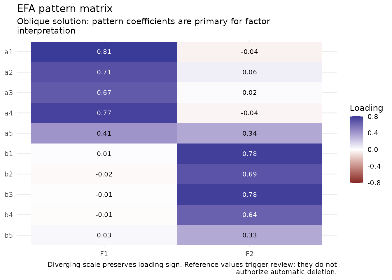

Residual strain

A plausible loading pattern can still leave localized relationships unexplained. nomo_efa() therefore returns the reproduced correlation matrix, the residual matrix, the off-diagonal RMSR, and ranked residual pairs.

efa$rmsr
#> [1] 0.01768766
head(efa$residual_pairs, 10)
#> # A tibble: 10 × 4
#>    item1 item2 residual abs_residual
#>    <chr> <chr>    <dbl>        <dbl>
#>  1 b4    b5      0.0425       0.0425
#>  2 a5    b5     -0.0388       0.0388
#>  3 a4    b5      0.0380       0.0380
#>  4 a2    a5      0.0295       0.0295
#>  5 b2    b5     -0.0277       0.0277
#>  6 a3    b5     -0.0272       0.0272
#>  7 a3    a4      0.0268       0.0268
#>  8 a4    b1      0.0264       0.0264
#>  9 a3    b4      0.0241       0.0241
#> 10 a4    b3     -0.0206       0.0206

plot(efa, type = "residuals")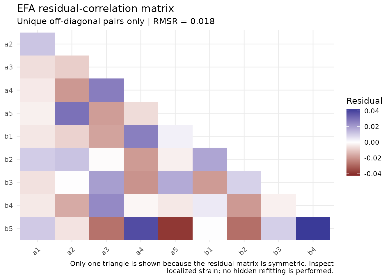

Residuals are diagnostic evidence. nomologR does not search for a better model, add correlated residuals, change the factor count, or remove indicators behind the user’s back.

Researcher control remains explicit

The default is common-factor MINRES extraction with oblimin rotation. Researchers may choose another common-factor extraction or rotation, but those choices remain visible in the result and decision log.

efa_varimax <- nomo_efa(
  nomo_demo_continuous,
  factors = 2,
  rotation = "varimax"
)
efa_varimax$item_summary[, c("item", "primary_loading", "secondary_loading", "attention")]
#> # A tibble: 10 × 4
#>    item  primary_loading secondary_loading attention    
#>    <chr>           <dbl>             <dbl> <chr>        
#>  1 a1              0.777             0.139 KEEP         
#>  2 a2              0.705             0.223 KEEP         
#>  3 a3              0.653             0.166 KEEP         
#>  4 a4              0.742             0.137 KEEP         
#>  5 a5              0.479             0.420 REVIEW       
#>  6 b1              0.766             0.190 KEEP         
#>  7 b2              0.671             0.136 KEEP         
#>  8 b3              0.761             0.169 KEEP         
#>  9 b4              0.618             0.132 REVIEW       
#> 10 b5              0.330             0.103 STRONG REVIEW

An orthogonal rotation is permitted rather than prohibited, but it forces the factors to be uncorrelated even though A and B correlate .40 in the population. The decision log asks the researcher to justify that assumption.

Ordered response categories

Many rating scales produce ordered categories rather than continuous scores. nomo_demo_ordinal stores the same latent responses as five-category ordered factors, so nomologR uses polychoric correlations automatically:

fac_ord <- nomo_factors(nomo_demo_ordinal, seed = 2026)
fac_ord$correlation
#> [1] "polychoric"

efa_ord <- nomo_efa(nomo_demo_ordinal, factors = fac_ord)
efa_ord$item_summary[, c("item", "primary_loading", "secondary_loading", "attention")]
#> # A tibble: 10 × 4
#>    item  primary_loading secondary_loading attention    
#>    <chr>           <dbl>             <dbl> <chr>        
#>  1 a1              0.792          -0.0257  KEEP         
#>  2 a2              0.695           0.0437  KEEP         
#>  3 a3              0.650           0.0258  KEEP         
#>  4 a4              0.768          -0.0535  KEEP         
#>  5 a5              0.433           0.307   REVIEW       
#>  6 b1              0.765           0.00370 KEEP         
#>  7 b2              0.650          -0.00701 KEEP         
#>  8 b3              0.740           0.0167  KEEP         
#>  9 b4              0.658          -0.0279  KEEP         
#> 10 b5              0.359          -0.0283  STRONG REVIEW

When Likert-type responses are stored as integers instead of ordered factors, integer storage alone does not tell nomologR whether the researcher intends a continuous or ordinal model. Declare the modeling level explicitly. This chunk only illustrates the syntax, because the teaching data already store ordered factors:

efa_declared <- nomo_efa(
  my_likert_items,
  factors = 2,
  types = c(q1 = "ordinal", q2 = "ordinal", q3 = "ordinal", q4 = "ordinal")
)

What should happen next?

EFA contributes exploratory evidence about latent structure. A defensible measurement workflow still requires theoretical interpretation and, where feasible, confirmation on fresh or holdout data. Continue with From CFA to a defensible measurement model.

Research basis

The package’s EFA philosophy follows reviews that documented problematic historical defaults — principal components presented as factor analysis, eigenvalues greater than one, orthogonal rotation, and mechanical deletion — and recommended common-factor models, evidence-based retention, and oblique rotation when factors may correlate (Fabrigar et al., 1999; Conway & Huffcutt, 2003; Browne, 2001; Watkins, 2018). Parallel analysis originates with Horn (1965); the eigenvalue-greater-than-one rule with Guttman (1954) and Kaiser (1960). See the research basis article for full references and the broader historical-to-contemporary map.