Theory-Specified Nomological Networks with nomologR • nomologR

Why theory comes before the network

nomologR treats nomological evidence as a test of explicit theoretical predictions, not as a search for statistically significant relationships.

The intended sequence is:

establish a defensible measurement model;
specify the expected relations before inspecting the structural results;
fit the full model;
compare estimates and uncertainty with the prespecified theoretical region;
distinguish theory strain, imprecision, measurement problems, and post-hoc exploration.

The teaching study

nomo_demo_network simulates a validation study of an Agency measure. Two related constructs were also measured — Persistence and Social desirability — along with an observed Performance outcome.

The population model is known (see ?nomo_demo_network):

Agency predicts Persistence (standardized coefficient .45);
Agency predicts Performance (.40);
Persistence has no direct effect on Performance once Agency is accounted for (0);
Agency and Social desirability are unrelated (0).

In real research you would not know these values. They are shown here so you can see how nomologR evidence behaves when a prediction is right, when it is wrong, and when it is about a negligible relation.

Specify theory before looking at results

h <- nomo_hypotheses(
  "Agency -> Persistence" = positive(min = .20),
  "Agency <-> SocialDesirability" = negligible(within = c(-.15, .15)),
  "Agency -> Performance" = positive(),
  "Persistence -> Performance" = positive(min = .20)
)

h
#> <nomo_hypotheses> Theory-specified relations
#> 4 theory-specified relations
#> 
#> Every relation is on the standardized scale.
#>   ID  Relation                       Prediction  Region         Origin
#>   H1  Agency -> Persistence          positive    [0.2, +Inf)    a priori
#>   H2  Agency <-> SocialDesirability  negligible  [-0.15, 0.15]  a priori
#>   H3  Agency -> Performance          positive    (0, +Inf)      a priori
#>   H4  Persistence -> Performance     positive    [0.2, +Inf)    a priori

A -> B means a directed structural path. A <-> B means an association without asserting causal direction.

The fourth prediction is plausible-sounding — persistent people perform better — but it is not true in the population model. It is included on purpose.

The negligible-effect region of ±.15 for Social desirability is a researcher-specified smallest effect size of interest (SESOI). It must be justified by theory or study design before the analysis; nomologR never invents one. A bare negligible() records a theoretical expectation, but nomologR will refuse to treat p > .05 as confirmation of negligibility.

Fit the latent network

model <- nomo_model(list(
  Agency = c("ag1", "ag2", "ag3", "ag4"),
  Persistence = c("pe1", "pe2", "pe3", "pe4"),
  SocialDesirability = c("sd1", "sd2", "sd3")
))

net <- nomo_network(
  model,
  data = nomo_demo_network,
  hypotheses = h
)

net
#> <nomo_network> Nomological network
#> Primary sample: N = 800 | Converged: yes
#> Theory relations: 4 | Added to the model from hypotheses: 3
#> Measurement context: no configured measurement-context review signal was
#> triggered
#> 
#> Hypothesis evidence
#>   ID  Relation                       Estimate  95% CI           Concordance
#>   H1  Agency -> Persistence             0.458  [0.389, 0.526]   Concordant
#>   H2  Agency <-> SocialDesirability     0.008  [-0.079, 0.095]  Concordant
#>   H3  Agency -> Performance             0.418  [0.341, 0.495]   Concordant
#>   H4  Persistence -> Performance       -0.062  [-0.146, 0.022]  Inconsistent
#> 
#> Theory concordance, uncertainty, measurement quality, and replication are
#> distinct evidence streams. Statistical significance alone is not a validity
#> verdict.
nomo_table(net, "fit")
#> # A tibble: 1 × 7
#>   chisq    df pvalue   cfi   tli  rmsea   srmr
#>   <dbl> <dbl>  <dbl> <dbl> <dbl>  <dbl>  <dbl>
#> 1  61.6    51  0.147 0.997 0.996 0.0161 0.0205

The measurement model supplies only the factor definitions. Theory-specified paths absent from that model are added transparently, and the exact fitted syntax and unchanged lavaan fit remain available in the returned object.

Read relation-level evidence

evidence <- nomo_table(net, "hypotheses")
evidence[, c(
  "id", "relation", "theoretical_region", "estimate",
  "ci_lower", "ci_upper", "equivalence_supported", "concordance"
)]
#> # A tibble: 4 × 8
#>   id    relation                   theoretical_region estimate ci_lower ci_upper
#>   <chr> <chr>                      <chr>                 <dbl>    <dbl>    <dbl>
#> 1 H1    Agency -> Persistence      [0.2, +Inf)         0.458     0.389    0.526 
#> 2 H2    Agency <-> SocialDesirabi… [-0.15, 0.15]       0.00773  -0.0794   0.0948
#> 3 H3    Agency -> Performance      (0, +Inf)           0.418     0.341    0.495 
#> 4 H4    Persistence -> Performance [0.2, +Inf)        -0.0624   -0.146    0.0215
#> # ℹ 2 more variables: equivalence_supported <lgl>, concordance <chr>

Reading each row:

H1 (Agency -> Persistence): estimate 0.46, interval [0.39, 0.53], classified concordant with the prediction of at least .20.
H2 (Agency <-> SocialDesirability): estimate 0.01. The 90% equivalence interval [-0.07, 0.08] lies inside the ±.15 region, so the negligible prediction is supported by equivalence evidence — not merely by a non-significant p-value.
H3 (Agency -> Performance): estimate 0.42, classified concordant.
H4 (Persistence -> Performance): estimate -0.06, interval [-0.15, 0.02], classified inconsistent with the predicted region.

Every relation also retains its standard error, p-value, evidence scope, a-priori versus post-hoc provenance, and a measurement-context flag. The goal is not to produce a single “validity score.”

A marginal association is not a structural prediction

Why might a researcher have expected H4? Look at the simple correlation between a Persistence composite and Performance:

persistence_mean <- rowMeans(nomo_demo_network[, c("pe1", "pe2", "pe3", "pe4")])
cor(persistence_mean, nomo_demo_network$Performance)
#> [1] 0.1180501

The marginal correlation is positive, because both Persistence and Performance depend on Agency. The theory-specified path asks a different question: does Persistence predict Performance given Agency? It does not. Treating a table of observed correlations as the nomological network would have produced the wrong conclusion.

Negligible predictions and equivalence evidence

For:

negligible(within = c(-.15, .15))
#> $prediction
#> [1] "negligible"
#> 
#> $lower
#> [1] -0.15
#> 
#> $upper
#> [1] 0.15
#> 
#> $lower_inclusive
#> [1] TRUE
#> 
#> $upper_inclusive
#> [1] TRUE
#> 
#> $scale
#> [1] "standardized"
#> 
#> $origin
#> [1] "a_priori"
#> 
#> $magnitude_specified
#> [1] TRUE
#> 
#> $confirmable
#> [1] TRUE
#> 
#> attr(,"class")
#> [1] "nomo_expectation" "list"

the researcher has supplied a quantitative negligible-effect region. With the default equivalence_alpha = .05, nomo_network() evaluates a 90% equivalence confidence interval, corresponding to the two one-sided tests procedure. This is intentionally different from declaring a relation negligible because an ordinary null-hypothesis test was not significant.

Criterion and predictive evidence

Performance is an observed variable, while Agency is latent. The evidence table labels such relations explicitly:

evidence[, c("id", "relation", "evidence_scope")]
#> # A tibble: 4 × 3
#>   id    relation                      evidence_scope            
#>   <chr> <chr>                         <chr>                     
#> 1 H1    Agency -> Persistence         latent_structural         
#> 2 H2    Agency <-> SocialDesirability latent_association        
#> 3 H3    Agency -> Performance         latent_to_observed_outcome
#> 4 H4    Persistence -> Performance    latent_to_observed_outcome

Observed outcomes keep their observed-variable estimand; nomologR does not silently insert measurement-error corrections.

Measurement context

nomo_table(net, "measurement")
#> # A tibble: 1 × 8
#>   attention converged latent_constructs loading_review_flags
#>   <chr>     <lgl>                 <int>                <int>
#> 1 info      TRUE                      3                    0
#> # ℹ 4 more variables: negative_variance_flags <int>,
#> #   global_fit_review_flags <int>, engine_warning_count <int>,
#> #   observation <chr>

A relation can look inconsistent with theory because the estimated relationship truly differs from the prediction, or because weak measurement, improper solutions, poor fit, or large uncertainty limit what the structural result can say. The measurement context stays beside the theory evidence so the two are not confused.

Calibration and validation

An internal split can be created explicitly:

s <- nomo_split(nomo_demo_network, validation_prop = .40, seed = 2026)

net_rep <- nomo_network(
  model,
  data = s,
  hypotheses = h
)

replication <- nomo_table(net_rep, "replication")
replication[, c(
  "id", "relation", "primary_estimate", "validation_estimate",
  "validation_concordance", "replication_status"
)]
#> # A tibble: 4 × 6
#>   id    relation     primary_estimate validation_estimate validation_concordance
#>   <chr> <chr>                   <dbl>               <dbl> <chr>                 
#> 1 H1    Agency -> P…           0.472              0.441   concordant            
#> 2 H2    Agency <-> …          -0.0285             0.0531  directionally_concord…
#> 3 H3    Agency -> P…           0.448              0.369   concordant            
#> 4 H4    Persistence…          -0.101              0.00364 direction_concordant_…
#> # ℹ 1 more variable: replication_status <chr>

The calibration and validation subsets receive the same prespecified fitted model; nomologR does not respecify the validation model to rescue a primary result. Reading the statuses:

H1 and H3 are replicated_concordance and replicated_concordance.
H2 is mixed_or_inconclusive: with only 320 validation cases, the equivalence interval is too wide to confirm negligibility. Splitting a sample buys independence at the cost of precision.
H4 is sign_change_within_uncertainty. The population path is zero, and the two point estimates happen to differ in sign. Here neither sample’s confidence interval excludes zero, so the sign change is attributed to sampling uncertainty rather than to a substantive discrepancy.

A change in sign between samples needs care. Estimates scattered around a null relation differ in sign about half the time, so nomologR does not call a sign change a reversal from the point estimates. It reads the 95 percent confidence intervals:

Status	Intervals	Meaning
`sign_reversal`	Both exclude zero, on opposite sides	Each sample on its own supports a different direction
`direction_not_replicated`	Exactly one excludes zero	The other sample does not support that direction, nor establish the opposite
`sign_change_within_uncertainty`	Neither excludes zero	Neither sample distinguishes the relation from zero

None of these turns a non-significant path into evidence of no relation. That claim needs a negligible(within = ...) prediction with an equivalence region, the kind of prediction H2 makes (Lakens, Scheel, & Isager, 2018).

External validation data can instead be supplied with validation_data =, which is generally stronger evidence than an internal split.

Figures

plot(net, type = "effects")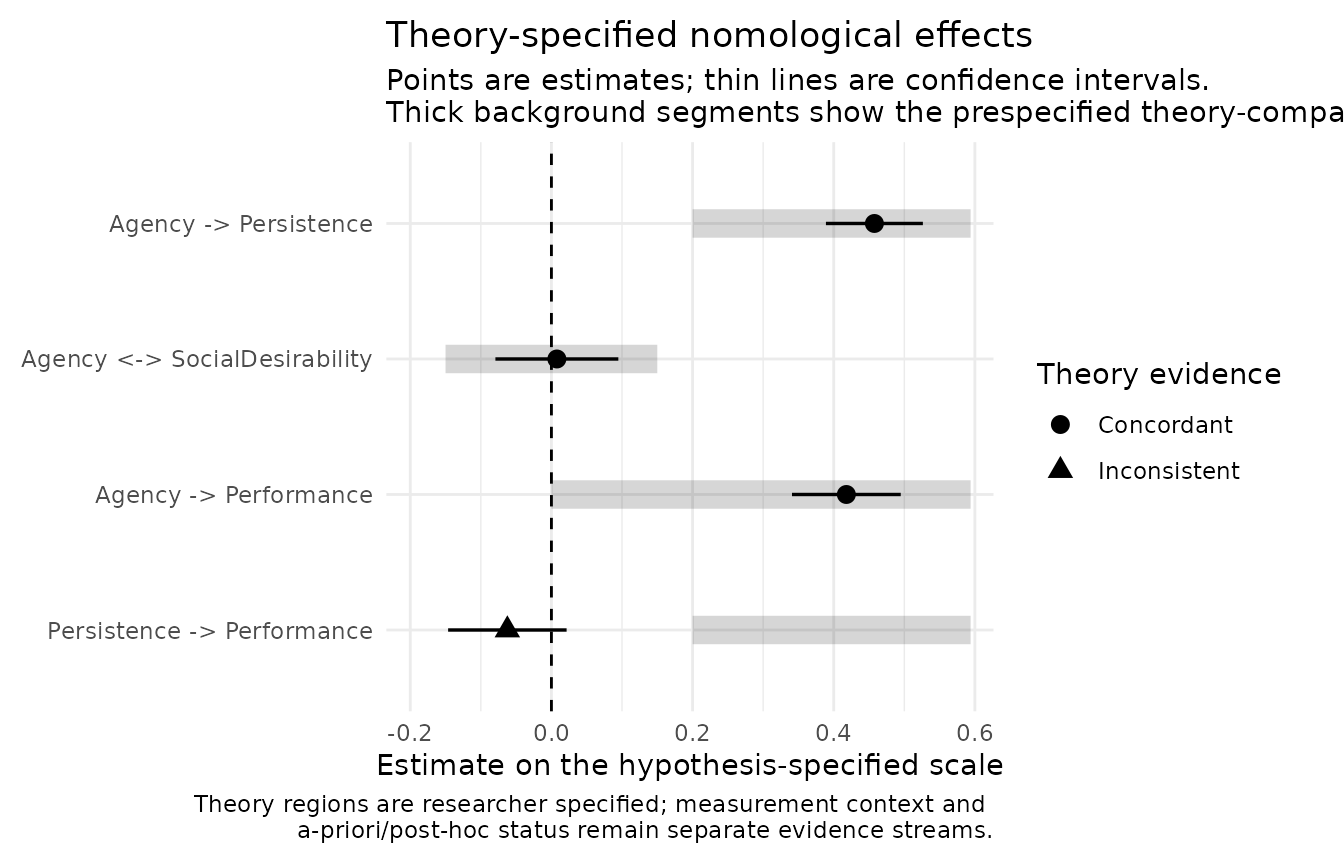

plot(net_rep, type = "replication")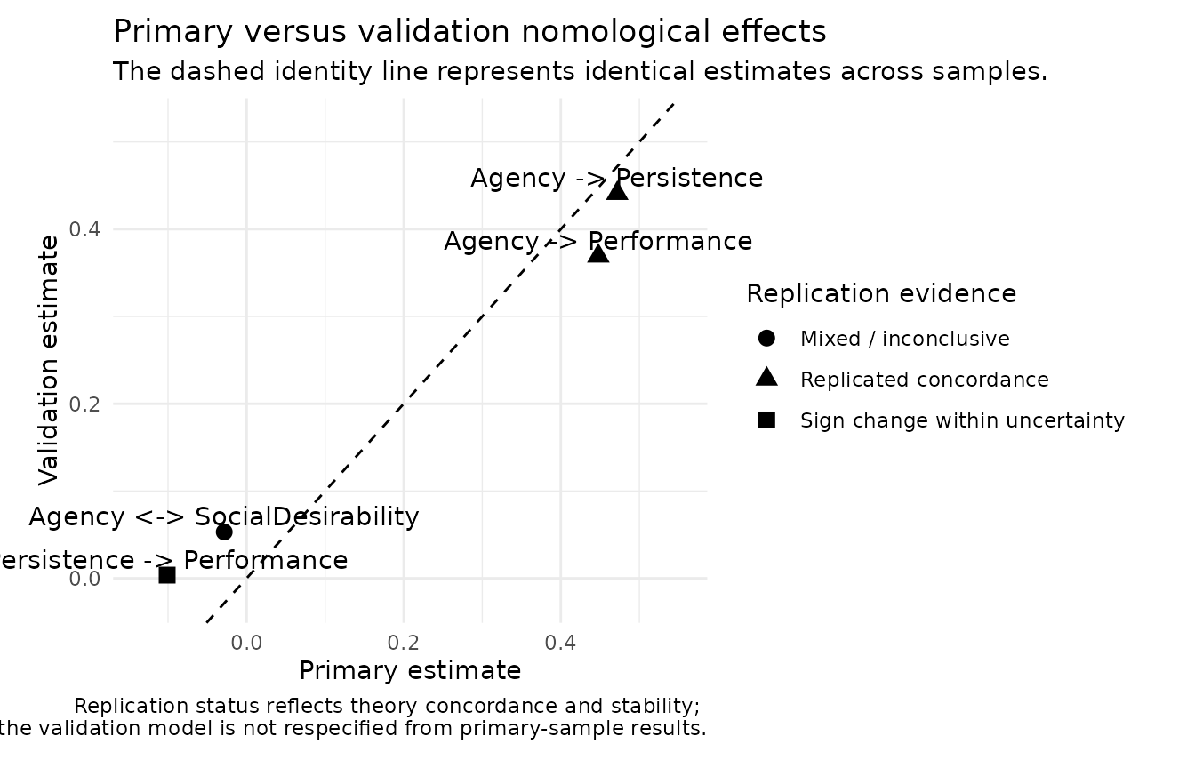

These are evidence summaries, not automated theory verdicts.

Interpretation rule

nomologR keeps measurement evidence, theory concordance, uncertainty, replication, and researcher provenance visible at the same time. A supported prediction strengthens the validity argument for a particular interpretation of scores; an unsupported one is information about the theory, the measure, or both.

Research basis

The nomological network as the core of construct validity comes from Cronbach and Meehl (1955), and convergent and discriminant correlation patterns from Campbell and Fiske (1959). Contemporary practice separates the measurement model from structural relations (Anderson & Gerbing, 1988), treats validity as an argument about score interpretation (Messick, 1995), evaluates negligible predictions with equivalence procedures (Schuirmann, 1987; Lakens, Scheel, & Isager, 2018), and distinguishes prespecified from post-hoc predictions (Nosek et al., 2018). Full references are in ?nomo_network and the research basis article.