From CFA to a defensible measurement model
Source:vignettes/measurement-model-evidence.Rmd
measurement-model-evidence.RmdWhy measurement evidence is staged
A confirmatory factor model, a reliability coefficient, and a
discriminant-validity statistic answer different questions. Treating
them as interchangeable checkboxes can produce misleading conclusions.
nomologR therefore keeps the workflow staged:
-
nomo_cfa()— Does the proposed measurement structure reproduce the data reasonably, and where is there model strain? -
nomo_reliability()— How consistently does the intended score represent its target under that measurement model? -
nomo_validity()— Do indicators converge on their intended constructs, and are theoretically distinct constructs empirically distinguishable?
The sequence is evidence-guided rather than pass/fail. A reference value can trigger inspection, but it never automatically deletes an indicator, merges constructs, or establishes construct validity.
A healthy two-factor model
We begin with a known two-factor population in which both factors are well measured and moderately correlated.
set.seed(2026)
n <- 500

f1 <- rnorm(n)
f2 <- .30 * f1 + sqrt(1 - .30^2) * rnorm(n)

healthy <- data.frame(
  A1 = .82 * f1 + rnorm(n, sd = .55),
  A2 = .79 * f1 + rnorm(n, sd = .58),
  A3 = .76 * f1 + rnorm(n, sd = .62),
  A4 = .80 * f1 + rnorm(n, sd = .57),
  B1 = .83 * f2 + rnorm(n, sd = .54),
  B2 = .78 * f2 + rnorm(n, sd = .60),
  B3 = .75 * f2 + rnorm(n, sd = .63),
  B4 = .81 * f2 + rnorm(n, sd = .56)
)

model <- '
  F1 =~ A1 + A2 + A3 + A4
  F2 =~ B1 + B2 + B3 + B4
'
cfa <- nomo_cfa(model, data = healthy)

# Modest resampling here keeps vignette build time reasonable.
# Use more resamples for final reporting.
rel <- nomo_reliability(
  cfa,
  ci = "bootstrap",
  ci_boot = 100,
  ci_seed = 2026
)
val <- nomo_validity(cfa, htmt = "both")
The compact summaries are intentionally different from the raw engine output. They surface the evidence most relevant to the user’s next decision without repeating the same full loading table in several places.
summary(rel)## <nomo_reliability summary> Reliability
##
## Coefficients
## Construct Indicators Omega Alpha
## F1 continuous 0.891 [0.871, 0.908] 0.890 [0.870, 0.907]
## F2 continuous 0.862 [0.840, 0.881] 0.861 [0.837, 0.881]
## Not shown for width: Omega scale. See nomo_table(x, "coefficients").
## Bracketed values are bootstrap confidence intervals.
##
## Omega is primary for the congeneric CFA workflow; alpha is secondary and
## assumption-dependent. Reliability contributes score-precision evidence, not
## construct validity.
summary(val)## <nomo_validity summary> Convergent and discriminant evidence
##
## Convergent evidence by construct
## Construct AVE Min |loading| Median |loading| Loadings flagged
## F1 0.671 0.793 0.822 0
## F2 0.611 0.711 0.795 0
##
## Construct separation
## Construct 1 Construct 2 Latent r 95% CI HTMT2 HTMT
## F1 F2 0.223 [0.127, 0.318] 0.221 0.225
##
## Standardized loadings and AVE address convergent evidence; latent correlations
## and HTMT-family statistics address construct separation. These are
## complementary questions, not interchangeable pass/fail tests.The figures also avoid duplication. Item-level loading evidence belongs to the CFA; reliability gets a coefficient plot; convergent validity gets an AVE plot; and construct separation gets an HTMT-family plot.
plot(cfa, type = "loadings")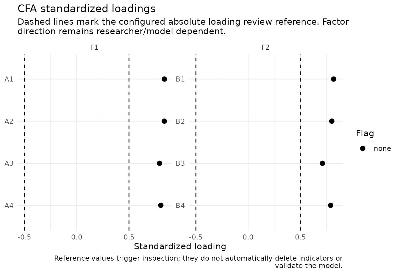
plot(rel)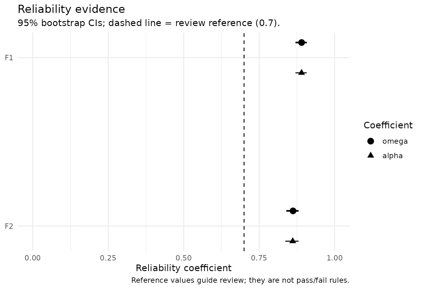
plot(val, type = "ave")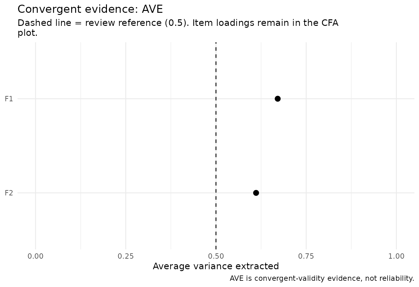
plot(val, type = "discriminant")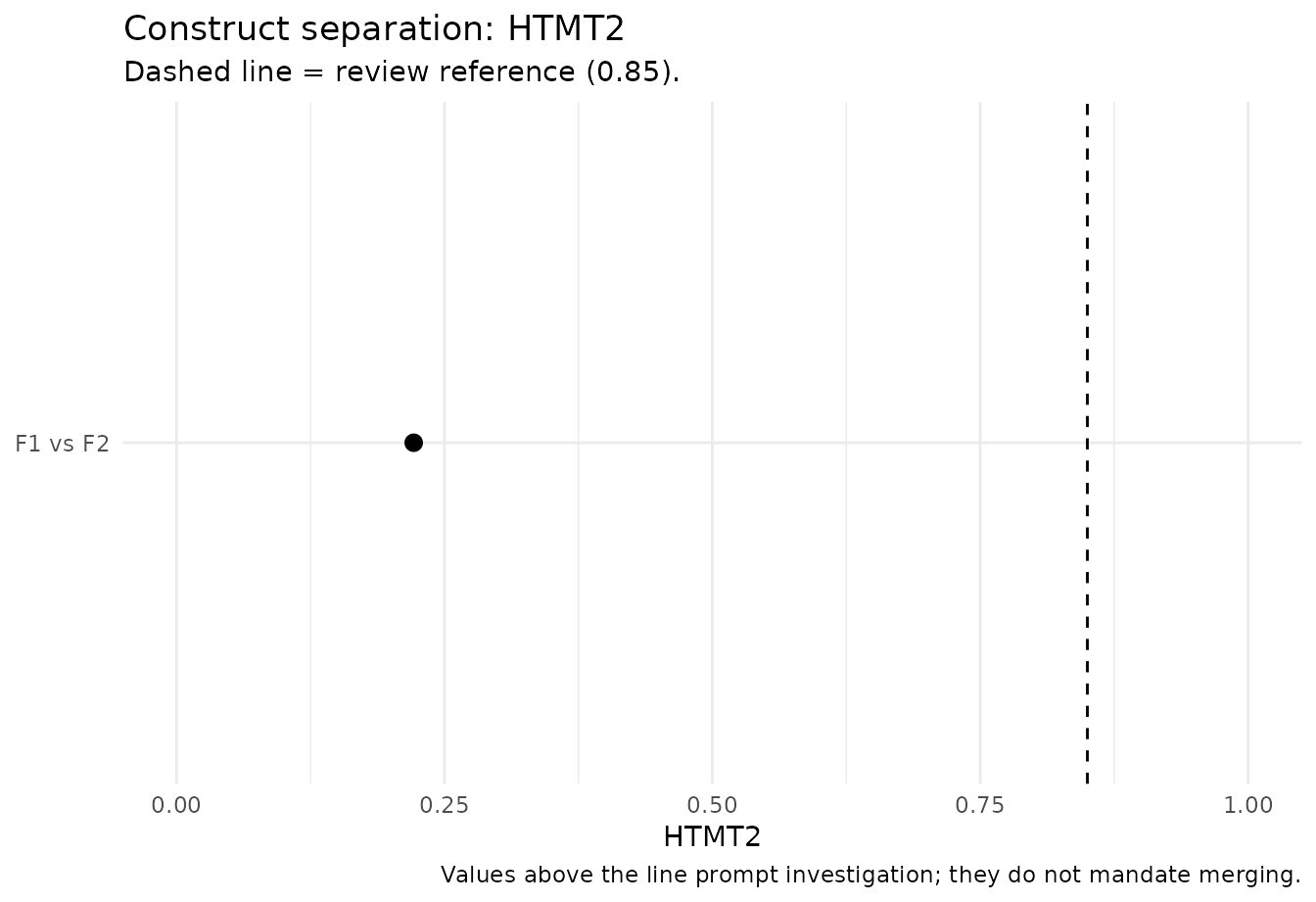
A healthy result contributes several complementary pieces of evidence. It does not turn the measurement model into a permanently “validated” object. Validity remains an accumulating argument tied to construct interpretation, population, setting, and intended use.
Good global fit does not guarantee good measurement
This is a critical teaching case. The following one-factor model is correctly specified, but its indicators are weak measures of the latent variable.
set.seed(2027)
n <- 650
f <- rnorm(n)

weak <- data.frame(
  W1 = .30 * f + rnorm(n, sd = .95),
  W2 = .34 * f + rnorm(n, sd = .94),
  W3 = .28 * f + rnorm(n, sd = .96),
  W4 = .32 * f + rnorm(n, sd = .95),
  W5 = .31 * f + rnorm(n, sd = .95)
)

weak_cfa <- nomo_cfa(
  'Weak =~ W1 + W2 + W3 + W4 + W5',
  data = weak
)
weak_rel <- nomo_reliability(weak_cfa)
weak_val <- nomo_validity(weak_cfa, htmt = "none")
weak_cfa$fit_evidence## # A tibble: 9 × 7
## metric value variant reference direction attention explanation
## <chr> <dbl> <chr> <dbl> <chr> <chr> <chr>
## 1 chi_square 2.79 chisq NA informat… info Descriptiv…
## 2 df 5 df NA informat… info Descriptiv…
## 3 p_value 0.733 pvalue NA informat… info Descriptiv…
## 4 CFI 1 cfi 0.95 higher info At or abov…
## 5 TLI 1.08 tli 0.95 higher info At or abov…
## 6 RMSEA 0 rmsea 0.06 lower info At or belo…
## 7 RMSEA_CI_lower 0 rmsea.ci.lower NA informat… info Descriptiv…
## 8 RMSEA_CI_upper 0.0393 rmsea.ci.upper NA informat… info Descriptiv…
## 9 SRMR 0.0152 srmr 0.08 lower info At or belo…Because the one-factor structure is the correct covariance model, global fit can look quite good. That does not imply that the items strongly represent the construct or that the resulting score is precise.
summary(weak_rel)## <nomo_reliability summary> Reliability
##
## Coefficients
## Construct Indicators Omega Alpha Omega scale Flag
## Weak continuous 0.369 0.363 observed continuous review
##
## Sampling uncertainty was not bootstrapped. For report-ready intervals, rerun
## with `ci = "bootstrap"`.
## Omega is primary for the congeneric CFA workflow; alpha is secondary and
## assumption-dependent. Reliability contributes score-precision evidence, not
## construct validity.
summary(weak_val)## <nomo_validity summary> Convergent and discriminant evidence
##
## Convergent evidence by construct
## Construct AVE Min |loading| Median |loading| Loadings flagged Flag
## Weak 0.114 0.200 0.311 5 review
##
## Construct separation
## No pairwise construct-separation summary is available.
##
## Standardized loadings and AVE address convergent evidence; latent correlations
## and HTMT-family statistics address construct separation. These are
## complementary questions, not interchangeable pass/fail tests.This is why nomologR does not collapse measurement
quality into a single global-fit verdict. Weak standardized loadings,
low AVE, and weak model-based reliability remain important even when
CFI, RMSEA, or SRMR look favorable.
Strong reliability does not guarantee construct separation
The reverse problem is also possible. Two constructs can each be measured very consistently while remaining difficult to distinguish empirically.
set.seed(2028)
n <- 700
f1 <- rnorm(n)
f2 <- .94 * f1 + sqrt(1 - .94^2) * rnorm(n)

overlap <- data.frame(
  A1 = .86 * f1 + rnorm(n, sd = .48),
  A2 = .83 * f1 + rnorm(n, sd = .51),
  A3 = .84 * f1 + rnorm(n, sd = .50),
  B1 = .86 * f2 + rnorm(n, sd = .48),
  B2 = .83 * f2 + rnorm(n, sd = .51),
  B3 = .84 * f2 + rnorm(n, sd = .50)
)

overlap_model <- '
  F1 =~ A1 + A2 + A3
  F2 =~ B1 + B2 + B3
'

overlap_cfa <- nomo_cfa(overlap_model, data = overlap)
overlap_rel <- nomo_reliability(overlap_cfa)
overlap_val <- nomo_validity(overlap_cfa, htmt = "both")
summary(overlap_rel)## <nomo_reliability summary> Reliability
##
## Coefficients
## Construct Indicators Omega Alpha Omega scale
## F1 continuous 0.893 0.894 observed continuous
## F2 continuous 0.896 0.895 observed continuous
##
## Sampling uncertainty was not bootstrapped. For report-ready intervals, rerun
## with `ci = "bootstrap"`.
## Omega is primary for the congeneric CFA workflow; alpha is secondary and
## assumption-dependent. Reliability contributes score-precision evidence, not
## construct validity.
summary(overlap_val)## <nomo_validity summary> Convergent and discriminant evidence
##
## Convergent evidence by construct
## Construct AVE Min |loading| Median |loading| Loadings flagged
## F1 0.737 0.837 0.865 0
## F2 0.742 0.848 0.851 0
##
## Construct separation
## Construct 1 Construct 2 Latent r 95% CI HTMT2 HTMT Flag
## F1 F2 0.933 [0.912, 0.954] 0.931 0.932 review
##
## Standardized loadings and AVE address convergent evidence; latent correlations
## and HTMT-family statistics address construct separation. These are
## complementary questions, not interchangeable pass/fail tests.Here, strong omega and AVE do not erase a high latent correlation or HTMT2 value. The package therefore recommends investigating theoretical distinctiveness, item content, cross-construct overlap, and the intended construct boundary. It does not automatically merge factors or delete indicators.
plot(overlap_val, type = "discriminant")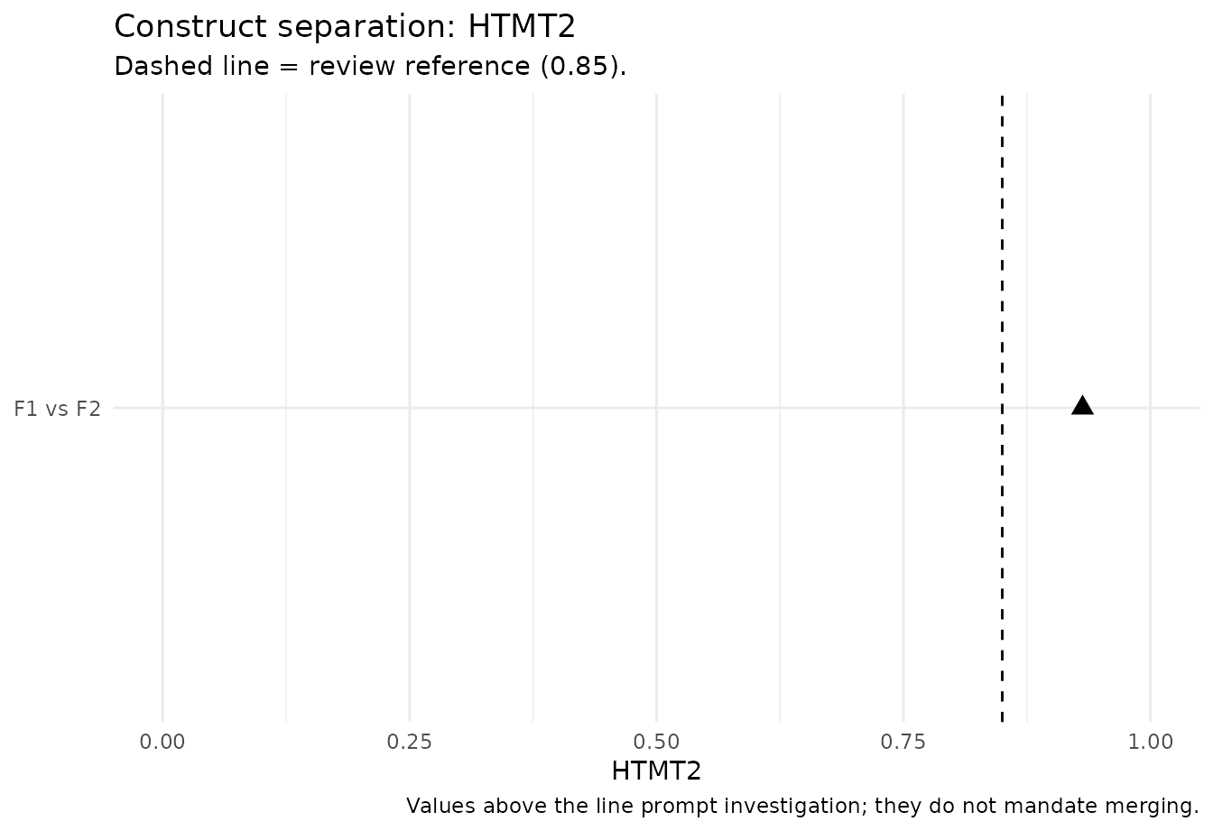
Ordered indicators: keep the score scale explicit
For ordered Likert-type indicators, nomo_cfa() uses an
ordered-data CFA workflow when the indicators are declared ordered.
nomo_reliability() then distinguishes the observed
ordinal-score reliability estimand from the hypothetical latent-response
scale.
set.seed(2029)
n <- 500
f <- rnorm(n)
z <- data.frame(
  I1 = .82 * f + rnorm(n, sd = .60),
  I2 = .79 * f + rnorm(n, sd = .62),
  I3 = .76 * f + rnorm(n, sd = .65),
  I4 = .80 * f + rnorm(n, sd = .60)
)

ordinal <- as.data.frame(lapply(z, function(x) {
  ordered(cut(x, breaks = c(-Inf, -.8, -.25, .25, .8, Inf), labels = 1:5))
}))

ordinal_cfa <- nomo_cfa(
  'F =~ I1 + I2 + I3 + I4',
  data = ordinal,
  ordered = names(ordinal)
)
ordinal_rel <- nomo_reliability(
  ordinal_cfa,
  ordinal_scale = TRUE,
  include_alpha = TRUE
)
summary(ordinal_rel)
## <nomo_reliability summary> Reliability
##
## Coefficients
## Construct Indicators Omega Omega scale
## F ordered 0.829 observed ordinal
##
## Secondary alpha unavailable for
## - F (ordered indicators, observed ordinal scale): Observed-scale alpha is
## not computed from an ordered-indicator CFA. Current semTools intentionally
## disallows ord.scale = TRUE with tau-equivalent alpha for ordered
## composites because that is a different scoring analysis from model-based
## ordinal reliability. Use the observed-scale omega estimate as the primary
## reliability evidence; calculate observed-score alpha separately only when
## that estimand is substantively required.
##
## Sampling uncertainty was not bootstrapped. For report-ready intervals, rerun
## with `ci = "bootstrap"`.
## Omega is primary for the congeneric CFA workflow; alpha is secondary and
## assumption-dependent. Reliability contributes score-precision evidence, not
## construct validity.Observed-scale omega is available for the practical ordinal composite. Observed-scale alpha is deliberately reported as unavailable in this ordered-CFA estimand rather than silently replacing it with a different definition. The point is not to maximize the number of coefficients reported; it is to keep the score and estimand clear.
Continuing the exploratory example
The exploratory walkthrough
flagged a cross-loading item (a5) and a weak item
(b5) in nomo_demo_continuous. Suppose the
researcher prespecifies the intended two-factor simple structure with
all ten items and fits it as a CFA:
demo_model <- nomo_model(list(
  A = c("a1", "a2", "a3", "a4", "a5"),
  B = c("b1", "b2", "b3", "b4", "b5")
))

demo_cfa <- nomo_cfa(demo_model, data = nomo_demo_continuous)
demo_cfa$fit_evidence
## # A tibble: 9 × 7
## metric value variant reference direction attention explanation
## <chr> <dbl> <chr> <dbl> <chr> <chr> <chr>
## 1 chi_square 75.8 chisq NA informat… info Descriptiv…
## 2 df 34 df NA informat… info Descriptiv…
## 3 p_value 0.0000500 pvalue NA informat… info Descriptiv…
## 4 CFI 0.973 cfi 0.95 higher info At or abov…
## 5 TLI 0.965 tli 0.95 higher info At or abov…
## 6 RMSEA 0.0510 rmsea 0.06 lower info At or belo…
## 7 RMSEA_CI_lower 0.0356 rmsea.ci.… NA informat… info Descriptiv…
## 8 RMSEA_CI_upper 0.0665 rmsea.ci.… NA informat… info Descriptiv…
## 9 SRMR 0.0519 srmr 0.08 lower info At or belo…
head(demo_cfa$top_modification_indices, 5)## # A tibble: 5 × 8
## lhs op rhs mi epc sepc.lv sepc.all sepc.nox
## <chr> <chr> <chr> <dbl> <dbl> <dbl> <dbl> <dbl>
## 1 B =~ a5 48.3 0.488 0.377 0.365 0.365
## 2 B =~ a1 9.41 -0.183 -0.141 -0.145 -0.145
## 3 a5 ~~ b3 7.57 0.0812 0.0812 0.150 0.150
## 4 a5 ~~ b1 4.78 0.0610 0.0610 0.125 0.125
## 5 a3 ~~ a4 4.64 0.0732 0.0732 0.133 0.133Three lessons carry over from the exploratory stage:
-
Modification indices are quarantined. The largest
index points toward the cross-loading that the data-generating model
contains, but
nomologRdoes not add it. Allowing a cross-loading, revising the item, or evaluating a model without it is a theoretical decision; freeing parameters because an index is large is capitalization on chance (MacCallum, Roznowski, & Necowitz, 1992). -
The same sample is not independent confirmation.
This CFA uses the data that suggested the structure.
nomo_split()or a new sample provides a stronger test. -
Missing data are handled explicitly. By default
lavaan uses complete cases here;
missing = "fiml"requests full-information maximum likelihood for continuous indicators, and the decision is recorded. Whether the results depend on that choice is a separate question, taken up below.
Comparing models with a recorded rationale
nomo_compare() evaluates competing measurement models
side by side. It requires a rationale, checks whether the models are
nested, reports the difference test that matches the estimator when they
are, and never selects a model automatically.
A cross-loading suggested by the results
The largest modification index above pointed to a loading of
a5 on factor B. Because that idea came from the results
rather than from theory stated in advance, the comparison is labeled
post hoc:
cross_cfa <- nomo_cfa(
  "A =~ a1 + a2 + a3 + a4 + a5\nB =~ b1 + b2 + b3 + b4 + b5 + a5",
  data = nomo_demo_continuous
)

cross_comparison <- nomo_compare(
  simple_structure = demo_cfa,
  cross_loading = cross_cfa,
  rationale = "The largest modification index suggested that a5 also reflects factor B.",
  origin = "post_hoc"
)
cross_comparison
## <nomo_compare> Measurement-model comparison
## Models: 2 | Reference: simple_structure | Estimator: ML | Cases: 473
## Origin: post-hoc
## Rationale: The largest modification index suggested that a5 also reflects
## factor B.
##
## Compared with `simple_structure`
## - cross_loading (nested, less constrained): chi-square difference = 48.72,
## df = 1, p < .001; CFI change +0.027, RMSEA change -0.051; AIC change -46.7
##
## No model was selected automatically. summary() shows interpretations and
## measurement evidence.Estimating the cross-loading reduces misfit (chi-square difference =
48.7, df = 1, p < .001; CFI changes by +0.027). That is exactly the
feature built into these simulated data, but with real data the evidence
alone does not settle the question. Does the wording of a5
plausibly reflect both constructs? Because the comparison is post hoc,
the decision log records it as such and recommends confirming the
retained model in independent data.
Is a weak item needed?
b5 loads weakly on B. Dropping b5 from the
model changes the data being modeled, so a model without the column
cannot be tested against the full model. Instead, keep b5
and fix its loading to zero:
b5_zero_cfa <- nomo_cfa(
  "A =~ a1 + a2 + a3 + a4 + a5\nB =~ b1 + b2 + b3 + b4 + 0*b5",
  data = nomo_demo_continuous
)

b5_comparison <- nomo_compare(
  full = demo_cfa,
  b5_loading_zero = b5_zero_cfa,
  rationale = paste(
    "Evaluate whether the weakly loading item b5 contributes to factor B",
    "before deciding whether to keep it."
  )
)
summary(b5_comparison)
## <nomo_compare summary> Measurement-model comparison
## Rationale: Evaluate whether the weakly loading item b5 contributes to factor B
## before deciding whether to keep it.
## Origin: a-priori | Reference model: full
##
## Model fit
## Model Parameters df Chi-square CFI TLI RMSEA SRMR
## full 21 34 75.83 0.973 0.965 0.051 0.052
## b5_loading_zero 20 35 122.75 0.944 0.928 0.073 0.093
##
## Information criteria
## Model AIC BIC Loadings fixed to zero
## full 11981.0 12068.4 0
## b5_loading_zero 12025.9 12109.1 1
##
## Difference tests against the reference model
## Model Relation Check Method Chi-sq diff df
## b5_loading_zero nested, more constrained nested standard 46.91 1
## Not shown for width: p. See nomo_table(x, "comparisons").
##
## Changes in fit (model minus reference)
## Model CFI TLI RMSEA SRMR AIC BIC
## b5_loading_zero -0.029 -0.036 +0.022 +0.042 +44.9 +40.8
##
## Interpretation
## - `b5_loading_zero` is nested within `full` and has 1 more degree of freedom
## (additional constraints). Chi-Squared Difference Test: chi-square
## difference = 46.91, df = 1, p < .001. A small p-value indicates that the
## extra constraints are not fully consistent with the data; with large
## samples, even small misspecifications produce small p-values. Change in
## fit (`b5_loading_zero` minus `full`): CFI -0.029, TLI -0.036, RMSEA
## +0.022, SRMR +0.042. AIC +44.9 and BIC +40.8 (`b5_loading_zero` minus
## `full`); lower values favor a model for these data, and only differences
## are interpretable. No model is selected automatically; read this evidence
## with theory and the recorded rationale.
##
## Standardized loadings by model
## Factor Item full b5_loading_zero
## A a1 0.771 0.771
## A a2 0.744 0.744
## A a3 0.669 0.669
## A a4 0.738 0.738
## A a5 0.598 0.598
## B b1 0.794 0.795
## B b2 0.695 0.699
## B b3 0.757 0.757
## B b4 0.628 0.624
## B b5 0.337 0.000
##
## Measurement evidence by model
## Construct Metric full b5_loading_zero
## A omega 0.835 0.835
## B omega 0.784 0.622
## A alpha 0.827 0.827
## B alpha 0.771 0.771
## A AVE 0.497 0.497
## B AVE 0.434 0.521
## B vs A HTMT2 0.533 0.533
## - The loading fixed to zero for b5 keeps that item in this composite; the
## coefficient does not describe a shortened scale.
##
## No model was selected automatically. Difference tests, changes in fit,
## information criteria, and measurement evidence answer different questions;
## read them together with theory and the recorded rationale.Fixing the loading to zero worsens fit (chi-square difference = 46.9,
df = 1, p < .001), so b5 is statistically related to B.
Its standardized loading, however, is only 0.34. With 473 cases, even a
weak relation is detectable; statistical detectability is not the same
as an adequate indicator. The decision still depends on whether
b5 covers content the construct needs.
plot(b5_comparison, type = "loadings")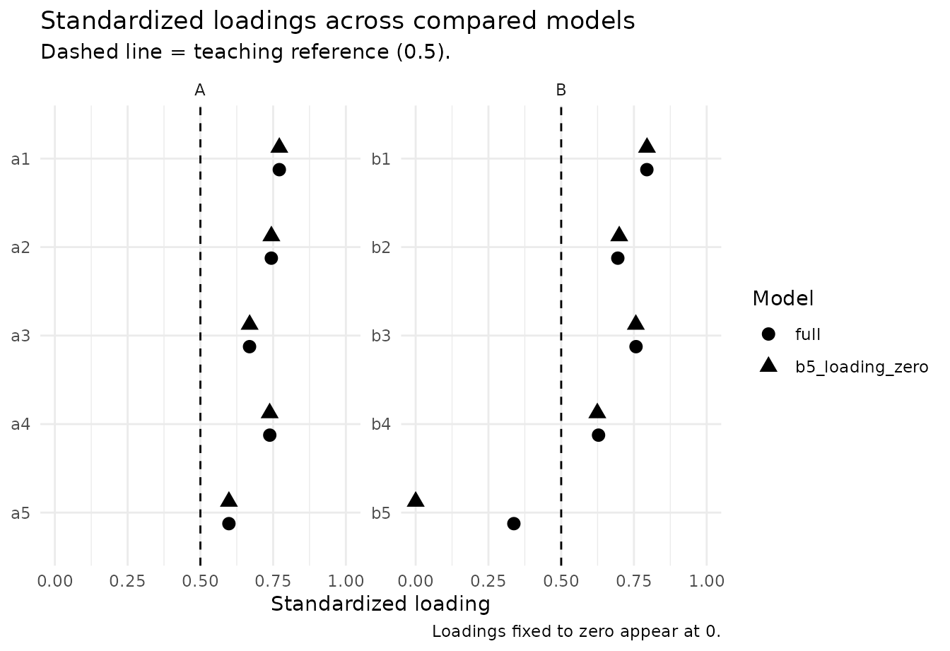
The summary’s measurement evidence carries a note: omega for B in the
zero-loading model still includes b5 in the composite, so
it does not describe a shortened four-item scale. To see that scale’s
reliability, fit the model without b5. Because the two
models contain different observed variables, nomo_compare()
reports this comparison descriptively, without a difference test or
information criteria:
shortened_cfa <- nomo_cfa(
  "A =~ a1 + a2 + a3 + a4 + a5\nB =~ b1 + b2 + b3 + b4",
  data = nomo_demo_continuous
)

shortened <- nomo_compare(
  full = demo_cfa,
  four_item_b = shortened_cfa,
  rationale = "Describe the reliability of a four-item B scale alongside the full scale."
)

nomo_table(shortened, "comparisons")[, c("model", "relation", "test_available", "ic_available")]
## # A tibble: 1 × 4
## model relation test_available ic_available
## <chr> <chr> <lgl> <lgl>
## 1 four_item_b different_variables FALSE FALSE
omega_rows <- nomo_table(shortened, "evidence")
omega_rows[omega_rows$metric == "omega", c("model", "construct", "estimate")]
## # A tibble: 4 × 3
## model construct estimate
## <chr> <chr> <dbl>
## 1 full A 0.835
## 2 full B 0.784
## 3 four_item_b A 0.835
## 4 four_item_b B 0.812Together these results separate three questions that are easy to blur: whether an item is statistically related to its factor, whether it is a strong indicator, and how the score’s reliability changes without it. None of them alone decides whether the item stays.
Does a result depend on how missing data were handled?
demo_cfa used lavaan’s default, listwise deletion, which
analyses only the cases observed on every item.
nomo_missing() refits the same model under alternative
strategies and reports what changes. For continuous indicators it
compares listwise deletion with full-information maximum likelihood
(FIML), which uses every observed response:
demo_missing <- nomo_missing(demo_cfa, data = nomo_demo_continuous)
demo_missing
## <nomo_missing> Missing-data sensitivity
## Model: nomo_cfa | Reference: FIML | Fitted with: Listwise deletion
## Cases: 27 of 500 incomplete (5.4%) | Patterns: 3
## Lowest covariance coverage: 0.946 (a2, b3)
##
## Strategies
## Strategy lavaan Needs Role N Converged Admissible
## Listwise deletion listwise MCAR comparison 473 yes yes
## FIML ml MAR reference 500 yes yes
##
## Largest differences from the reference, in reference standard errors
## Parameter Strategy Estimate Reference Difference (SE)
## A ~~ B Listwise deletion 0.499 0.480 +0.45
## B =~ b5 Listwise deletion 0.337 0.353 -0.37
## A =~ a5 Listwise deletion 0.598 0.590 +0.23
## A =~ a3 Listwise deletion 0.669 0.675 -0.21
## B =~ b3 Listwise deletion 0.757 0.762 -0.17
##
## Whether data are missing at random cannot be tested from these data; see
## nomo_table(x, "decision_log").The two strategies make different assumptions. Listwise deletion requires data missing completely at random (MCAR). FIML requires the weaker condition that data are missing at random (MAR), meaning that whether a value is missing may depend on other observed values but not on the missing value itself. In Enders and Bandalos’s (2001) simulations, all of these methods were unbiased under MCAR, and FIML was the most efficient. Under MAR, FIML alone remained unbiased across the parameters they examined.
The missing values in nomo_demo_continuous were
introduced completely at random, so theory predicts agreement, and that
is what the comparison shows. Listwise deletion discards 27 cases. No
estimate moves by as much as half a standard error. That is the size
Schafer and Graham (2002) treat as practically important for bias,
because beyond it confidence intervals noticeably lose coverage.
Reliability barely moves either:
nomo_table(demo_missing, "reliability")## # A tibble: 8 × 8
## construct block metric strategy role estimate reference_estimate difference
## <chr> <chr> <chr> <chr> <chr> <dbl> <dbl> <dbl>
## 1 A overall omega listwise comp… 0.835 0.835 -0.000589
## 2 A overall omega ml refe… 0.835 0.835 NA
## 3 B overall omega listwise comp… 0.784 0.785 -0.00151
## 4 B overall omega ml refe… 0.785 0.785 NA
## 5 A overall alpha listwise comp… 0.827 0.828 -0.000358
## 6 A overall alpha ml refe… 0.828 0.828 NA
## 7 B overall alpha listwise comp… 0.771 0.775 -0.00328
## 8 B overall alpha ml refe… 0.775 0.775 NAWhen the strategies disagree
Differences appear when data are missing at random but not completely at random. In this simulation the population factor correlation is .50. Most cases with high scores on factor A are missing every B item, so whether B is missing depends on the observed A items:
set.seed(32)
n <- 4000
f <- matrix(rnorm(n * 2), n, 2) %*% chol(matrix(c(1, .5, .5, 1), 2))
items <- cbind(
  f[, 1] %o% rep(.7, 4) + matrix(rnorm(n * 4, sd = sqrt(1 - .7^2)), n),
  f[, 2] %o% rep(.7, 4) + matrix(rnorm(n * 4, sd = sqrt(1 - .7^2)), n)
)
mar_data <- as.data.frame(items)
names(mar_data) <- c(paste0("a", 1:4), paste0("b", 1:4))

high_a <- rowMeans(mar_data[, paste0("a", 1:4)]) > 0
drop <- high_a & runif(n) < .90
mar_data[drop, paste0("b", 1:4)] <- NA

mar_model <- "A =~ a1 + a2 + a3 + a4\nB =~ b1 + b2 + b3 + b4"
mar_missing <- nomo_missing(
  nomo_cfa(mar_model, data = mar_data),
  data = mar_data,
  reliability = FALSE
)

mar_estimates <- nomo_table(mar_missing, "estimates")
mar_estimates[mar_estimates$type == "factor_correlation",
              c("strategy", "estimate", "se", "difference_in_se")]
## # A tibble: 2 × 4
## strategy estimate se difference_in_se
## <chr> <dbl> <dbl> <dbl>
## 1 listwise 0.411 0.0264 -2.01
## 2 ml 0.467 0.0280 NAFIML’s estimate, 0.467, is 1.2 of its standard errors from the population value, within sampling error. Listwise deletion’s, 0.411, is 3.4 standard errors below it. The complete cases under-represent high scorers on A, and that restricted range attenuates the correlation. The decision log flags the difference and says what it can and cannot mean:
mar_log <- nomo_table(mar_missing, "decision_log")
mar_log$recommendation[mar_log$metric == "estimate_difference"]
## [1] "If the data are MAR and the model is correct, FIML is consistent and this difference estimates the bias listwise deletion introduces; Schafer and Graham (2002) treat a bias of this size as practically important. Listwise deletion analyses 1789 fewer cases than the fullest strategy (44.7%), and the more cases a strategy discards, the larger the differences that sampling variability alone produces. Report which strategy the results rest on and why."The flag carries two qualifications:
- The difference estimates listwise deletion’s bias only if the data are MAR and the model is correct, because only then is FIML consistent.
- The two strategies analyze different cases, so part of any difference is sampling variability. The more cases listwise deletion discards, the larger that part becomes.
What the comparison cannot tell you
Whether data are MAR cannot, in general, be tested from the data at
hand (Schafer & Graham, 2002). Agreement between strategies
therefore shows only that a result does not depend on the choice between
them. It does not show that either strategy is unbiased: when data are
missing not at random, neither is guaranteed to be. The strategy belongs
in the analysis plan, decided in advance, and
nomo_missing() reports how much the results depend on
it.
For ordered indicators estimated with WLSMV, lavaan does not offer
FIML, so nomo_missing() compares listwise with pairwise
deletion. Both require MCAR, so a difference between them shows that the
result depends on the choice, but it cannot be attributed to either
strategy.
Mean substitution is not offered. Replacing each missing value with the item mean shrinks variances and distorts covariances. Schafer and Graham (2002) show that even under MCAR it narrows confidence intervals: with a quarter of values missing, a nominal 95% interval for a mean covers the true value only about 86% of the time. Multiple imputation, which Schafer and Graham recommend alongside maximum likelihood, is a candidate for a later release.
Reading the evidence as an argument
A useful measurement conclusion is rarely “all cutoffs passed.” A stronger conclusion identifies what each analysis contributes and what remains uncertain. The workflow is therefore designed around four questions:
- Structure: Is the hypothesized factor model a reasonable representation of the data?
- Precision: Is the intended score sufficiently reliable for its use, conditional on that model?
- Convergence: Do indicators substantially represent the intended construct?
- Separation: Are constructs that theory distinguishes also distinguishable empirically?
The resulting decision logs preserve observations, references, recommendations, and researcher decisions without automatically changing the scale or model.
Research basis
The reliability workflow follows the literature recommending
model-based omega for congeneric measurement and cautioning against
mechanical use of coefficient alpha, including Dunn, Baguley, and
Brunsden (2014), Flora (2020), and Bell, Chalmers, and Flora (2024).
Ordered-score reliability follows the distinction emphasized by Green
and Yang (2009) and implemented in semTools.
The validity workflow treats AVE as convergent evidence rather than reliability, following Fornell and Larcker (1981). For construct separation, HTMT-family evidence is prioritized because simulation research shows that older criteria can miss overlap (Henseler, Ringle, & Sarstedt, 2015). HTMT2 is emphasized for congeneric measurement because it relaxes the original HTMT tau-equivalence assumption (Roemer, Schuberth, & Henseler, 2021). Fornell-Larcker output remains available only as optional historical/ supporting information.
The missing-data comparison follows Enders and Bandalos (2001), whose simulations compared FIML with listwise and pairwise deletion under MCAR and MAR, and Schafer and Graham (2002), who review the older methods and explain why MAR cannot be tested from the data at hand.
The research basis article places
each of these methods between historical and contemporary practice, and
nomo_methods(stage = c("cfa", "compare", "reliability", "validity"))
returns the same information as a table, with full references.