Total and subscale scores: bifactor and higher-order models • nomologR

Many published scales report a total score and several subscale scores. A correlated-factors CFA can show that the subscales are distinguishable, but it cannot say whether a total score is defensible, or how much a subscale score adds once the total is known. Those questions need a model with a general factor and indices that divide each score’s variance between the general factor and the subscales.

This article shows how nomologR fits and evaluates the two common models for that purpose, and why model fit alone cannot choose between them.

Two ways to model a general factor

A higher-order model has first-order factors, one per subscale, whose correlations are explained by a second-order factor. The general factor reaches the items only through the first-order factors.
A bifactor model has a general factor measured directly by every item, plus a group factor for each subscale. All factors are orthogonal, so each item’s variance divides cleanly between the general factor, its group factor, and error.

The bifactor model dates to Holzinger and Swineford (1937), and Schmid and Leiman (1957) showed how to re-express a higher-order solution in bifactor form. Bifactor models were later rediscovered as a way to evaluate multidimensional measures (Reise, 2012), with indices for judging total and subscale scores (Reise, Bonifay, & Haviland, 2013; Rodriguez, Reise, & Haviland, 2016). The research basis article places these methods in context.

An example with a general factor

The data below are simulated from a bifactor population: twelve items in three four-item subscales, with a general factor that every item reflects and a weaker group factor for each subscale.

simulate_from <- function(sigma, n, seed) {
  set.seed(seed)
  z <- matrix(rnorm(n * ncol(sigma)), n, ncol(sigma))
  dat <- as.data.frame(z %*% chol(sigma))
  names(dat) <- colnames(sigma)
  dat
}

items <- paste0("x", 1:12)
subscale <- rep(1:3, each = 4)
general_loading <- c(.70, .60, .65, .55, .60, .50, .70, .60, .50, .60, .55, .65)
group_loading <- c(.40, .50, .30, .45, .50, .35, .40, .30, .45, .40, .50, .35)

L <- cbind(
  general_loading,
  sapply(1:3, function(k) ifelse(subscale == k, group_loading, 0))
)
sigma_bifactor <- L %*% t(L)
diag(sigma_bifactor) <- 1
dimnames(sigma_bifactor) <- list(items, items)

dat <- simulate_from(sigma_bifactor, n = 600, seed = 2026)

nomo_model() writes the syntax for all three structures from the same list of subscales. The researcher chooses the structure; nomologR never derives one from exploratory results.

subscales <- list(
  Focus = paste0("x", 1:4),
  Drive = paste0("x", 5:8),
  Poise = paste0("x", 9:12)
)

nomo_model(subscales, structure = "bifactor", general = "G")
#> G =~ NA*x1 + x2 + x3 + x4 + x5 + x6 + x7 + x8 + x9 + x10 + x11 + x12
#> Focus =~ NA*x1 + x2 + x3 + x4
#> Drive =~ NA*x5 + x6 + x7 + x8
#> Poise =~ NA*x9 + x10 + x11 + x12
#> G ~~ 1*G
#> Focus ~~ 1*Focus
#> Drive ~~ 1*Drive
#> Poise ~~ 1*Poise
#> G ~~ 0*Focus + 0*Drive + 0*Poise
#> Focus ~~ 0*Drive + 0*Poise
#> Drive ~~ 0*Poise

The bifactor syntax states its identification explicitly: each factor’s first loading is freed, each factor’s variance is fixed to 1, and every covariance among factors is fixed to 0. A higher-order model with three first-order factors carries a note that matters later:

nomo_model(subscales, structure = "higher_order", general = "G")
#> Focus =~ x1 + x2 + x3 + x4
#> Drive =~ x5 + x6 + x7 + x8
#> Poise =~ x9 + x10 + x11 + x12
#> G =~ NA*Focus + Drive + Poise
#> G ~~ 1*G
#> 
#> Identification notes:
#> - With three first-order factors the second-order part is just identified: this model fits exactly as well as the correlated-factors model, so model fit cannot distinguish the two.

correlated <- nomo_cfa(nomo_model(subscales), data = dat)
higher <- nomo_cfa(nomo_model(subscales, "higher_order"), data = dat)
bifactor <- nomo_cfa(nomo_model(subscales, "bifactor"), data = dat)

How much of each score is general?

nomo_hierarchical() reads the structure from the fitted model and reports the indices:

h <- nomo_hierarchical(bifactor)
h
#> <nomo_hierarchical> Hierarchical model evaluation
#> Bifactor model | General factor: G | Group factors: Focus, Drive, Poise
#> Estimand: unit-weighted observed composite
#> 
#> Total score
#>   Index                        Estimate
#>   omega total                     0.915
#>   omega hierarchical              0.792
#>   omega hierarchical relative     0.865
#>   ECV                             0.676
#>   PUC                             0.727
#> 
#> Subscales
#>   Subscale  Items  Omega subscale  Omega hierarchical subscale
#>   Focus         4           0.839                        0.288
#>   Drive         4           0.819                        0.204
#>   Poise         4           0.807                        0.295
#> 
#> Factor scores
#>   Factor  Role     Determinacy  Min competing r  Replicability H
#>   G       general        0.898            0.612            0.878
#>   Focus   group          0.709            0.007            0.500
#>   Drive   group          0.639           -0.185            0.403
#>   Poise   group          0.699           -0.022            0.485
#> 
#> Notes
#>   - review: A bifactor model will usually fit at least as well as
#>     correlated-factors or higher-order models of the same items, even when it
#>     did not generate the data (Reise, 2012), and a higher-order model is a
#>     constrained version of it (Yung, Thissen, & McLeod, 1999). Bonifay, Lane,
#>     and Reise (2017) call the bifactor model's tendency to show superior
#>     goodness of fit in model comparison studies a particular concern, and say
#>     that superior fit may be a symptom of overfitting: modeling not only the
#>     trends in the data but also unwanted noise. Murray and Johnson (2013)
#>     compared these two structures directly and found the comparison biased in
#>     favor of the bifactor model: unless there was essentially no unmodeled
#>     complexity, their simulation favored the bifactor model even when a
#>     higher-order model generated the data. They concluded that which model to
#>     adopt should not rely on which is better fitting. Compare the alternatives
#>     with nomo_compare() and choose on substantive grounds, not on fit alone.
#>   - review: Factor determinacy is at or below .90 for G, Focus, Drive, Poise.
#>     Gorsuch (1983, p. 260) recommended using factor score estimates only above
#>     that value. This is his recommendation reported as context, not a rule
#>     applied here; the score may still be usable for some purposes.
#>   - review: Two equally valid sets of factor scores could correlate as low as
#>     G (0.61), Focus (0.01), Drive (-0.18), Poise (-0.02). Gorsuch (1983, p.
#>     260) suggested this minimum be above .70. A negative value means two
#>     researchers scoring the same data could rank people in opposite orders and
#>     both be consistent with the model.
#>   - review: Construct replicability H is below .70 for Focus, Drive, Poise.
#>     Hancock and Mueller (2001) proposed .70 as a standard; a factor below it
#>     is not well defined by its own indicators and is expected to change across
#>     studies. Reported as their standard, not applied as a rule.
#> 
#> No index is treated as a pass/fail threshold; see nomo_table(x, "indices").

Reading the total score:

Omega total (0.92) is the proportion of total-score variance explained by all common factors.
Omega hierarchical (0.79) is the part explained by the general factor alone. It is the index that speaks to interpreting the total score as a measure of one construct.
Their ratio (0.86) says how much of the total score’s reliable variance is general.
ECV (0.68) is the share of common item variance the general factor explains, and PUC (0.73) is the share of item correlations influenced only by the general factor.

The subscales tell a different story:

nomo_table(h, "subscales")[, c(
  "subscale", "omega_subscale", "omega_hierarchical_subscale"
)]
#> # A tibble: 3 × 3
#>   subscale omega_subscale omega_hierarchical_subscale
#>   <chr>             <dbl>                       <dbl>
#> 1 Focus             0.839                       0.288
#> 2 Drive             0.819                       0.204
#> 3 Poise             0.807                       0.295

Focus has an omega of 0.84, which looks like a reliable subscale. But its omega hierarchical subscale is 0.29: once the general factor is removed, that is the reliable variance specific to Focus. Only 0.34 of a Focus score’s reliable variance is specific to Focus; the rest is the general factor, which the total score already measures. Reise, Bonifay, and Haviland (2013) frame exactly this question: whether subscale scores are justified, and how much reliable variance they add after controlling for the general factor.

The same division is shown for every composite:

plot(h)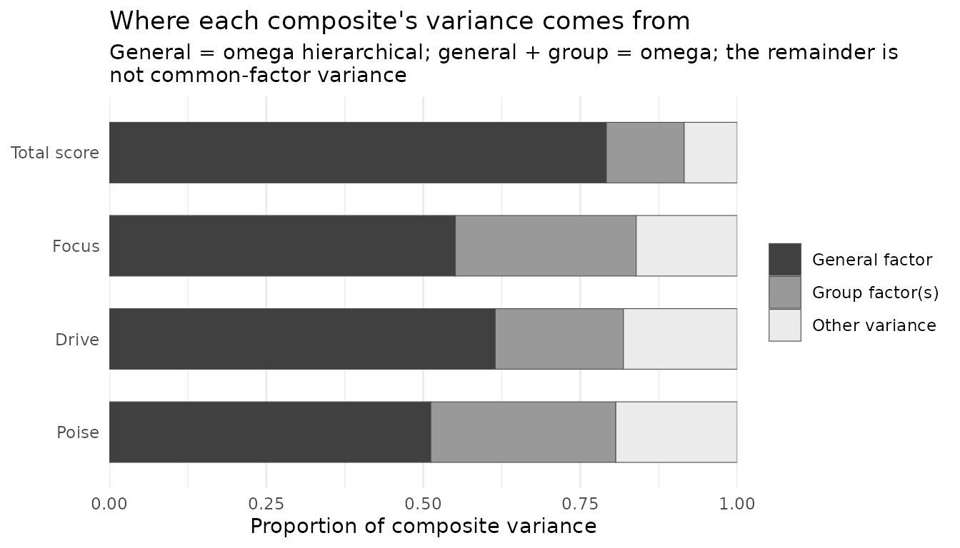

nomologR does not turn these indices into verdicts. Published heuristic values exist, but Reise (2012) notes that no benchmark value of ECV establishes when a general factor is strong enough. Whether a subscale score is worth reporting depends on its intended use, and the indices are the evidence for that decision rather than the decision itself.

Can you score the factors?

The omega indices describe unit-weighted composites: the sum score a researcher would actually compute. A different question is how well each factor can be recovered at all. The factors table answers it two ways:

nomo_table(h, "factors")
#> # A tibble: 4 × 7
#>   factor role    n_items factor_determinacy determinacy_r2 min_competing_r
#>   <chr>  <chr>     <int>              <dbl>          <dbl>           <dbl>
#> 1 G      general      12              0.898          0.806         0.612  
#> 2 Focus  group         4              0.709          0.503         0.00660
#> 3 Drive  group         4              0.639          0.408        -0.185  
#> 4 Poise  group         4              0.699          0.489        -0.0222 
#> # ℹ 1 more variable: construct_replicability <dbl>

factor_determinacy is the correlation between a factor and its estimated factor score (Beauducel, 2011; Rodriguez, Reise, & Haviland, 2016). Gorsuch (1983) recommended using factor score estimates only above .90. min_competing_r is the lowest correlation two equally valid sets of scores could have. When it is negative, two researchers scoring the same data with equally defensible methods could rank people in opposite orders, and both would be consistent with the model.

construct_replicability, Hancock and Mueller’s (2001) H, is the proportion of variance in a factor its own indicators could explain if optimally weighted. They proposed .70 as a standard.

The two indices answer different questions, and the difference is easy to miss. They are the same quantity when a construct is unidimensional. Under a bifactor model they are not: determinacy is computed from the whole reproduced correlation matrix, so a group factor’s score can borrow the other items to partial out the general factor, while H sees only that factor’s own loadings and treats the rest of each item as uncorrelated residual. Rodriguez et al. (2016) state that the two can differ here and decline to prefer either, so nomologR reports both and names what each one measures.

Neither threshold is applied as a rule. They are reported as their authors’ recommendations where a value falls below them, in the same way fixed fit-index cutoffs are treated elsewhere in the package.

Comparing structures

The three models can be compared with nomo_compare(), which requires a rationale and never selects a model:

cmp <- nomo_compare(
  correlated, higher, bifactor,
  rationale = "Competing structures for the same twelve items.",
  origin = "a_priori"
)

comparisons <- nomo_table(cmp, "comparisons")[, c(
  "model", "relation", "chisq_diff", "df_diff", "delta_cfi"
)]
comparisons$delta_cfi <- round(comparisons$delta_cfi, 4)
comparisons
#> # A tibble: 2 × 5
#>   model    relation         chisq_diff df_diff delta_cfi
#>   <chr>    <chr>                 <dbl>   <dbl>     <dbl>
#> 1 higher   equivalent             NA        NA    0     
#> 2 bifactor less_constrained       23.0       9    0.0047

Two features of this table are structural rather than empirical:

The higher-order model is equivalent to the correlated-factors model: both have chi-square = 72.45 on 51 degrees of freedom. With three first-order factors, the second-order part is just identified, so it imposes no testable constraint. Fit cannot distinguish the two, which is what the note on the syntax warned.
The bifactor model is less constrained. A higher-order model is a constrained version of the bifactor model (Yung, Thissen, & McLeod, 1999), so the bifactor model can only fit as well or better.

Why fit cannot choose the structure

That last point has a consequence. The next data set is simulated from a higher-order population, so the higher-order model is the true one:

first_order <- c(.70, .65, .60, .75, .70, .60, .65, .70, .55, .70, .65, .60)
second_order <- c(.80, .70, .60)

F <- sapply(1:3, function(k) ifelse(subscale == k, first_order, 0))
phi <- second_order %*% t(second_order)
diag(phi) <- 1
sigma_higher <- F %*% phi %*% t(F)
diag(sigma_higher) <- 1
dimnames(sigma_higher) <- list(items, items)

dat_higher <- simulate_from(sigma_higher, n = 600, seed = 2027)

true_model <- nomo_cfa(nomo_model(subscales, "higher_order"), data = dat_higher)
bifactor_model <- nomo_cfa(nomo_model(subscales, "bifactor"), data = dat_higher)

The higher-order model generated these data, yet the bifactor model fits better: chi-square = 38.14 on 42 degrees of freedom, against 42.48 on 51 for the true model. That is not a sign that the bifactor model is correct. Its extra parameters absorb sampling noise, and it will usually fit at least as well as correlated-factors or higher-order models of the same items (Reise, 2012).

So the choice between structures has to rest on theory: is there a construct that every item measures directly, with subscale content as a secondary source? Or is the general construct what the subscales have in common? Fit comparison can reveal a structure that clearly does not work, but it cannot make this choice.

Higher-order models and Schmid-Leiman

nomo_hierarchical() also evaluates higher-order models. There the group sources are the first-order factors’ disturbances, and the item loadings are the Schmid-Leiman decomposition of the higher-order solution, which is exact for a confirmatory model:

h_higher <- nomo_hierarchical(true_model)
nomo_table(h_higher, "indices")[, c("index", "estimate")]
#> # A tibble: 5 × 2
#>   index                       estimate
#>   <chr>                          <dbl>
#> 1 omega_total                    0.845
#> 2 omega_hierarchical             0.617
#> 3 omega_hierarchical_relative    0.730
#> 4 ecv                            0.481
#> 5 puc                            0.727
head(nomo_table(h_higher, "loadings"), 4)
#> # A tibble: 4 × 6
#>   item  subscale general_loading group_loading communality item_ecv
#>   <chr> <chr>              <dbl>         <dbl>       <dbl>    <dbl>
#> 1 x1    Focus              0.515         0.433       0.453    0.586
#> 2 x2    Focus              0.482         0.405       0.396    0.586
#> 3 x3    Focus              0.477         0.401       0.388    0.586
#> 4 x4    Focus              0.609         0.512       0.633    0.586

Each item’s general loading is its first-order loading multiplied by its factor’s second-order loading. Every item in a subscale therefore has the same ratio of general to group loading, which is why item_ecv is identical for all four Focus items. That proportionality is the constraint that distinguishes a higher-order model from a bifactor model, where each item’s split between general and group variance is free.

Ordered indicators

When indicators are declared ordered, nomo_cfa() fits the model with WLSMV and nomo_hierarchical() computes the indices on the latent-response scale. Those omegas are upper bounds on the reliability of the observed ordinal sum score, and the output says so. The observed ordinal-scale versions are not provided.

What nomologR does not do

It does not generate a bifactor or higher-order structure from exploratory results. The researcher specifies the structure.
It does not apply pass/fail thresholds to omega hierarchical, ECV, or PUC.
It does not choose between correlated-factors, higher-order, and bifactor models, and it discloses that fit comparisons favor the bifactor model.
It evaluates single-group, single-level models, and refuses models whose general and group factors are allowed to correlate, because variance cannot then be attributed to a source.

Every method used here is listed, with references, by nomo_methods():

nomo_methods(h)[, c("method", "lineage", "role")]
#> # A tibble: 7 × 3
#>   method                                    lineage      role      
#>   <chr>                                     <chr>        <chr>     
#> 1 Bifactor measurement model                contemporary primary   
#> 2 Omega hierarchical                        contemporary primary   
#> 3 Omega hierarchical subscale               contemporary supporting
#> 4 Explained common variance                 contemporary supporting
#> 5 Factor determinacy                        contemporary supporting
#> 6 Construct replicability (H)               contemporary supporting
#> 7 Percentage of uncontaminated correlations contemporary supporting

References

Holzinger, K. J., & Swineford, F. (1937). The bi-factor method. Psychometrika, 2(1), 41–54. https://doi.org/10.1007/BF02287965

Reise, S. P. (2012). The rediscovery of bifactor measurement models. Multivariate Behavioral Research, 47(5), 667–696. https://doi.org/10.1080/00273171.2012.715555

Reise, S. P., Bonifay, W. E., & Haviland, M. G. (2013). Scoring and modeling psychological measures in the presence of multidimensionality. Journal of Personality Assessment, 95(2), 129–140. https://doi.org/10.1080/00223891.2012.725437

Rodriguez, A., Reise, S. P., & Haviland, M. G. (2016). Evaluating bifactor models: Calculating and interpreting statistical indices. Psychological Methods, 21(2), 137–150. https://doi.org/10.1037/met0000045

Schmid, J., & Leiman, J. M. (1957). The development of hierarchical factor solutions. Psychometrika, 22(1), 53–61. https://doi.org/10.1007/BF02289209

Yung, Y.-F., Thissen, D., & McLeod, L. D. (1999). On the relationship between the higher-order factor model and the hierarchical factor model. Psychometrika, 64(2), 113–128. https://doi.org/10.1007/BF02294531