Compare confirmatory measurement models

nomo_compare() places two or more fitted nomo_cfa() models side by side and reports the evidence that bears on the comparison: a difference test matched to the estimator when the models are nested, changes in global fit indices, information criteria when they are defined, and standardized loadings, reliability, and construct-separation evidence for each model. A researcher rationale is required and recorded. The function never selects a "winning" model.

Usage

nomo_compare(
  ...,
  rationale,
  origin = c("a_priori", "post_hoc"),
  nested = c("auto", "yes", "no"),
  reference = 1L,
  method = "default",
  evidence = TRUE,
  guidance = nomo_defaults()
)

Arguments

...

Two or more nomo_cfa objects. Argument names become model labels, for example nomo_compare(full = cfa_full, reduced = cfa_reduced, rationale = "...").

rationale

Required character scalar recording why these models are compared (for example, the theoretical question each model represents).

origin

Whether the comparison was planned before seeing results ("a_priori") or prompted by results such as modification indices or residuals ("post_hoc"). Post-hoc comparisons are flagged in the decision log.

nested

"auto" (default) checks nesting automatically; "yes" declares the models nested; "no" declares them non-nested and skips the difference test.

reference

The model every other model is compared with, as an index or label. Defaults to the first model.

method

Difference-test method passed to lavaan::lavTestLRT(). "default" lets lavaan choose the method appropriate to the estimator.

evidence

Logical. If TRUE (default), compute side-by-side reliability (nomo_reliability()) and convergent/discriminant (nomo_validity()) evidence for each model.

guidance

Guidance settings from nomo_defaults().

Value

A nomo_compare object. The fields to read are:

• models: fit and information criteria for each model.

• comparisons: for each model against the reference, the nesting relation, the difference test, changes in fit and information criteria, and an interpretation.

• loadings: standardized loadings side by side.

• evidence: reliability, AVE, and HTMT2 by model, when evidence = TRUE.

• fits: the fitted nomo_cfa objects, and engine_warnings, the warnings lavaan raised for each.

• reference, rationale, origin, references, and decision_log.

Other fields record the call, the settings used, and intermediate engine results. They may change between releases and are not part of the stable interface (see ?nomologR).

Details

Requirements. All models must be converged nomo_cfa objects fitted with the same estimator and missing-data handling to the same cases and data. Otherwise the comparison is refused with an explanation, because test statistics and fit indices would not be comparable.

Nesting. With nested = "auto", nesting is checked from the models' implied moments with semTools::net() (Bentler & Satorra, 2010). The difference test is reported only for nested models. If the check cannot run (for example for some categorical models), set nested = "yes" when one model is obtained from the other by fixing or constraining parameters. A declaration that the check contradicts is recorded as a concern and no test is reported.

Difference tests. Tests come from lavaan::lavTestLRT(): the ordinary chi-square difference test for ML, the scaled difference test for robust ML estimators (Satorra & Bentler, 2001), and the scaled-and-shifted test for categorical estimators such as WLSMV (Satorra, 2000). The method lavaan used is reported. A test that lavaan cannot compute, or a negative scaled statistic, is reported as unavailable with lavaan's message rather than replaced by a different method; method can request an alternative explicitly.

Information criteria. AIC and BIC are reported for likelihood-based estimators when the models contain the same observed variables. They are not defined for WLSMV and are reported as unavailable, not substituted.

Removing an item. Models with different observed variables describe different data, so neither a difference test nor information criteria applies; only descriptive evidence is shown. To test whether an item is needed, keep it in both models and fix its loading to zero in the reduced model (for example B =~ b1 + b2 + b3 + b4 + 0*b5). Reliability for such a model still includes the zero-loading item in the composite, and the evidence table says so.

References

Akaike, H. (1974). A new look at the statistical model identification. IEEE Transactions on Automatic Control, 19(6), 716-723. doi:10.1109/TAC.1974.1100705

Bentler, P. M., & Satorra, A. (2010). Testing model nesting and equivalence. Psychological Methods, 15(2), 111-123. doi:10.1037/a0019625

Burnham, K. P., & Anderson, D. R. (2004). Multimodel inference: Understanding AIC and BIC in model selection. Sociological Methods & Research, 33(2), 261-304. doi:10.1177/0049124104268644

Chen, F. F. (2007). Sensitivity of goodness of fit indexes to lack of measurement invariance. Structural Equation Modeling, 14(3), 464-504. doi:10.1080/10705510701301834

Cheung, G. W., & Rensvold, R. B. (2002). Evaluating goodness-of-fit indexes for testing measurement invariance. Structural Equation Modeling, 9(2), 233-255. doi:10.1207/S15328007SEM0902_5

MacCallum, R. C., Roznowski, M., & Necowitz, L. B. (1992). Model modifications in covariance structure analysis: The problem of capitalization on chance. Psychological Bulletin, 111(3), 490-504. doi:10.1037/0033-2909.111.3.490

Raftery, A. E. (1995). Bayesian model selection in social research. Sociological Methodology, 25, 111-163. doi:10.2307/271063

Satorra, A. (2000). Scaled and adjusted restricted tests in multi-sample analysis of moment structures. In Innovations in multivariate statistical analysis (pp. 233-247). Springer. doi:10.1007/978-1-4615-4603-0_17

Satorra, A., & Bentler, P. M. (2001). A scaled difference chi-square test statistic for moment structure analysis. Psychometrika, 66(4), 507-514. doi:10.1007/BF02296192

Satorra, A., & Bentler, P. M. (2010). Ensuring positiveness of the scaled difference chi-square test statistic. Psychometrika, 75(2), 243-248. doi:10.1007/s11336-009-9135-y

Schwarz, G. (1978). Estimating the dimension of a model. The Annals of Statistics, 6(2), 461-464. doi:10.1214/aos/1176344136

See also

nomo_cfa() to fit the models.

Examples

full <- nomo_cfa(
  "A =~ a1 + a2 + a3 + a4 + a5\nB =~ b1 + b2 + b3 + b4 + b5",
  data = nomo_demo_continuous
)
# Keep b5 in the data but fix its loading to zero to test whether it is needed
no_b5 <- nomo_cfa(
  "A =~ a1 + a2 + a3 + a4 + a5\nB =~ b1 + b2 + b3 + b4 + 0*b5",
  data = nomo_demo_continuous
)

cmp <- nomo_compare(
  full = full,
  no_b5 = no_b5,
  rationale = "Evaluate whether the weakly loading item b5 contributes to factor B.",
  evidence = FALSE
)
cmp
#> <nomo_compare> Measurement-model comparison
#> Models: 2 | Reference: full | Estimator: ML | Cases: 473 | Origin: a-priori
#> Rationale: Evaluate whether the weakly loading item b5 contributes to factor
#> B.
#> 
#> Compared with `full`
#>   - no_b5 (nested, more constrained): chi-square difference = 46.91, df = 1, p
#>     < .001; CFI change -0.029, RMSEA change +0.022; AIC change +44.9
#> 
#> No model was selected automatically. summary() shows interpretations and
#> measurement evidence.
nomo_table(cmp, "comparisons")
#> # A tibble: 1 × 23
#>   model reference relation    nested_declared nesting_check nested df_difference
#>   <chr> <chr>     <chr>       <chr>           <chr>         <lgl>          <dbl>
#> 1 no_b5 full      more_const… auto            nested        TRUE               1
#> # ℹ 16 more variables: test <chr>, method <chr>, chisq_diff <dbl>,
#> #   df_diff <dbl>, p_value <dbl>, test_available <lgl>, test_note <chr>,
#> #   delta_cfi <dbl>, delta_tli <dbl>, delta_rmsea <dbl>, delta_srmr <dbl>,
#> #   delta_aic <dbl>, delta_bic <dbl>, ic_available <lgl>, ic_note <chr>,
#> #   interpretation <chr>

# \donttest{
# Side-by-side loadings, reliability, AVE, and HTMT2 for each model
cmp_evidence <- nomo_compare(
  full = full,
  no_b5 = no_b5,
  rationale = "Evaluate whether the weakly loading item b5 contributes to factor B."
)
summary(cmp_evidence)
#> <nomo_compare summary> Measurement-model comparison
#> Rationale: Evaluate whether the weakly loading item b5 contributes to factor
#> B.
#> Origin: a-priori | Reference model: full
#> 
#> Model fit
#>   Model  Parameters  df  Chi-square    CFI    TLI  RMSEA   SRMR
#>   full           21  34       75.83  0.973  0.965  0.051  0.052
#>   no_b5          20  35      122.75  0.944  0.928  0.073  0.093
#> 
#> Information criteria
#>   Model      AIC      BIC  Loadings fixed to zero
#>   full   11981.0  12068.4                       0
#>   no_b5  12025.9  12109.1                       1
#> 
#> Difference tests against the reference model
#>   Model  Relation                  Check   Method    Chi-sq diff  df       p
#>   no_b5  nested, more constrained  nested  standard        46.91   1  < .001
#> 
#> Changes in fit (model minus reference)
#>   Model     CFI     TLI   RMSEA    SRMR    AIC    BIC
#>   no_b5  -0.029  -0.036  +0.022  +0.042  +44.9  +40.8
#> 
#> Interpretation
#>   - `no_b5` is nested within `full` and has 1 more degree of freedom
#>     (additional constraints). Chi-Squared Difference Test: chi-square
#>     difference = 46.91, df = 1, p < .001. A small p-value indicates that the
#>     extra constraints are not fully consistent with the data; with large
#>     samples, even small misspecifications produce small p-values. Change in
#>     fit (`no_b5` minus `full`): CFI -0.029, TLI -0.036, RMSEA +0.022, SRMR
#>     +0.042. AIC +44.9 and BIC +40.8 (`no_b5` minus `full`); lower values favor
#>     a model for these data, and only differences are interpretable. No model
#>     is selected automatically; read this evidence with theory and the recorded
#>     rationale.
#> 
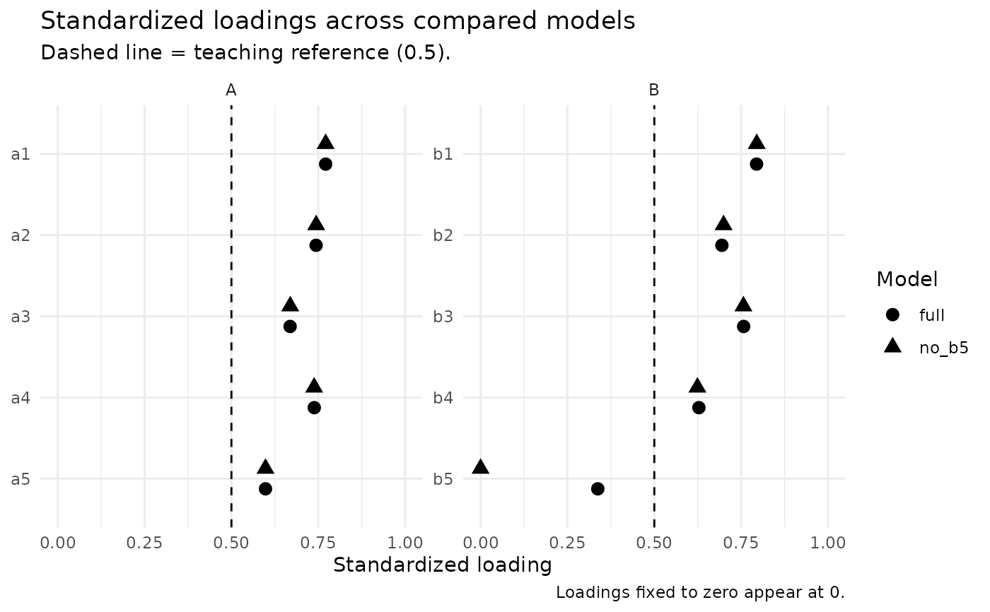
#> Standardized loadings by model
#>   Factor  Item   full  no_b5
#>   A       a1    0.771  0.771
#>   A       a2    0.744  0.744
#>   A       a3    0.669  0.669
#>   A       a4    0.738  0.738
#>   A       a5    0.598  0.598
#>   B       b1    0.794  0.795
#>   B       b2    0.695  0.699
#>   B       b3    0.757  0.757
#>   B       b4    0.628  0.624
#>   B       b5    0.337  0.000
#> 
#> Measurement evidence by model
#>   Construct  Metric   full  no_b5
#>   A          omega   0.835  0.835
#>   B          omega   0.784  0.622
#>   A          alpha   0.827  0.827
#>   B          alpha   0.771  0.771
#>   A          AVE     0.497  0.497
#>   B          AVE     0.434  0.521
#>   B vs A     HTMT2   0.533  0.533
#>   - The loading fixed to zero for b5 keeps that item in this composite; the
#>     coefficient does not describe a shortened scale.
#> 
#> No model was selected automatically. Difference tests, changes in fit,
#> information criteria, and measurement evidence answer different questions;
#> read them together with theory and the recorded rationale.
plot(cmp_evidence, type = "loadings")

# }