Measurement Invariance with nomologR • nomologR

What invariance is for

Measurement invariance asks whether a construct is measured comparably across groups or occasions. If it is not, a difference in observed scores can reflect how an item functions in each group rather than a difference in the construct itself. nomologR treats invariance as graded evidence rather than a sequence of automatic PASS/FAIL decisions.

Every fitted level retains:

the generated semTools::measEq.syntax() object and the exact lavaan syntax;
the fitted lavaan object;
absolute fit and change in fit;
nested-model comparison evidence where available;
localized equality-constraint diagnostics;
researcher-specified partial-invariance provenance.

A teaching example with a known answer

nomo_demo_network contains 800 responses collected in two administration groups, online and paper. Its population model builds in two features:

the latent Agency mean is .25 SD higher in the paper group (a real construct difference); and
the intercept of item ag3 is .50 higher in the paper group (item bias: ag3 is endorsed more on paper at the same level of Agency).

All loadings are equal across groups.

aggregate(
  cbind(ag1, ag2, ag3, ag4) ~ group,
  data = nomo_demo_network,
  FUN = mean
)
#>    group     ag1      ag2      ag3      ag4
#> 1 online 3.98885 3.971875 3.974900 4.027750
#> 2  paper 4.23735 4.252500 4.640525 4.265525

Every item mean is higher in the paper group, but ag3 is higher by much more. Observed means alone cannot separate the real latent difference from the item-level bias; that is the job of the invariance sequence.

Continuous indicators

agency_model <- "Agency =~ ag1 + ag2 + ag3 + ag4"

inv <- nomo_invariance(
  agency_model,
  data = nomo_demo_network,
  group = "group"
)

inv
#> <nomo_invariance> Measurement invariance
#> Grouping variable: group (2 groups: online, paper) | Indicators: continuous
#> Requested: configural -> metric -> scalar -> strict
#> Completed: configural -> metric -> scalar -> strict
#> 
#>   Level         CFI  RMSEA   SRMR  CFI change  RMSEA change   LRT p
#>   configural  1.000  0.000  0.002           -             -       -
#>   metric      1.000  0.000  0.028      +0.000        +0.000    .146
#>   scalar      0.954  0.121  0.065      -0.046        +0.121  < .001
#>   strict      0.954  0.102  0.066      +0.000        -0.019    .483
#> Localized equality-constraint diagnostics retained: 24
#> 
#> Fit changes and score diagnostics are evidence. They are not pass/fail rules,
#> and nomologR never frees a parameter because of them.

The conventional continuous sequence is:

configural -> metric -> scalar -> strict

fit <- nomo_table(inv, "fit")
fit[, c("level", "constraints", "cfi", "rmsea", "srmr", "delta_cfi", "delta_rmsea", "lrt_p")]
#> # A tibble: 4 × 8
#>   level      constraints       cfi rmsea    srmr delta_cfi delta_rmsea     lrt_p
#>   <chr>      <chr>           <dbl> <dbl>   <dbl>     <dbl>       <dbl>     <dbl>
#> 1 configural none            1     0     0.00200 NA            NA      NA       
#> 2 metric     loadings        1     0     0.0275   0             0       1.46e- 1
#> 3 scalar     loadings, inte… 0.954 0.121 0.0647  -0.0462        0.121   1.20e-13
#> 4 strict     loadings, inte… 0.954 0.102 0.0659   0.000420     -0.0193  4.83e- 1

The configural and metric models fit closely, consistent with equal loadings. Adding intercept equality at the scalar level changes CFI by -0.046 and RMSEA by 0.121, and the likelihood-ratio test is very small (p = 1.2e-13). No single delta-CFI, delta-RMSEA, delta-SRMR, or chi-square rule is treated as universally decisive; the evidence is read together, in context.

plot(inv, type = "change")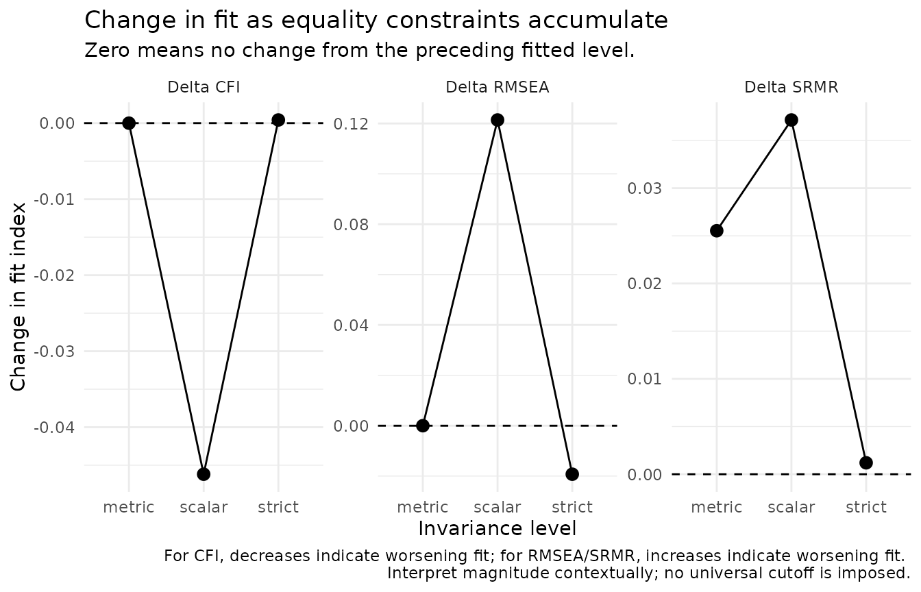

Localizing strain

Global change in fit says that a set of constraints is strained. Score diagnostics help locate where.

strain <- nomo_table(inv, "local_strain")
strain[, c("level", "constraint_display", "score_x2", "df", "p_value")]
#> # A tibble: 24 × 5
#>    level  constraint_display                        score_x2    df  p_value
#>    <chr>  <chr>                                        <dbl> <dbl>    <dbl>
#>  1 metric Loading: Agency -> ag3 (online vs. paper)   4.92       1 2.66e- 2
#>  2 metric Loading: Agency -> ag2 (online vs. paper)   1.03       1 3.10e- 1
#>  3 metric Loading: Agency -> ag4 (online vs. paper)   0.690      1 4.06e- 1
#>  4 metric Loading: Agency -> ag1 (online vs. paper)   0.0273     1 8.69e- 1
#>  5 scalar Intercept: ag3 (online vs. paper)          61.1        1 5.33e-15
#>  6 scalar Intercept: ag1 (online vs. paper)          11.3        1 7.68e- 4
#>  7 scalar Intercept: ag4 (online vs. paper)           5.56       1 1.83e- 2
#>  8 scalar Intercept: ag2 (online vs. paper)           0.977      1 3.23e- 1
#>  9 scalar Loading: Agency -> ag2 (online vs. paper)   0.546      1 4.60e- 1
#> 10 scalar Loading: Agency -> ag1 (online vs. paper)   0.317      1 5.74e- 1
#> # ℹ 14 more rows

plot(inv, type = "local_strain")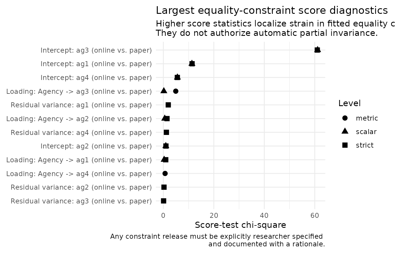

The largest scalar-level diagnostic is Intercept: ag3 (online vs. paper) (score chi-square 61.1), which matches the item bias built into the data.

Two cautions matter for real research:

Score diagnostics never authorize an automatic parameter release. With many constraints, some diagnostics will look notable by chance; look at the smaller metric-level values above for an example.
In real data you do not know the population model. A release chosen only because its diagnostic was largest is a post-hoc decision and should be reported as one.

Researcher-controlled partial invariance

release <- nomo_partial(
  level = "scalar",
  syntax = "ag3 ~ 1",
  rationale = paste(
    "The ag3 wording was expected to read differently on paper forms;",
    "this expectation was documented before the analysis."
  )
)

inv_partial <- nomo_invariance(
  agency_model,
  data = nomo_demo_network,
  group = "group",
  partial = release
)

nomo_table(inv_partial, "partial")
#> # A tibble: 1 × 4
#>   release_id level  syntax  rationale                                           
#>   <chr>      <chr>  <chr>   <chr>                                               
#> 1 P1         scalar ag3 ~ 1 The ag3 wording was expected to read differently on…

fit_partial <- nomo_table(inv_partial, "fit")
fit_partial[, c("level", "partial_requested", "cfi", "rmsea", "delta_cfi", "lrt_p")]
#> # A tibble: 4 × 6
#>   level      partial_requested   cfi rmsea delta_cfi  lrt_p
#>   <chr>      <chr>             <dbl> <dbl>     <dbl>  <dbl>
#> 1 configural ""                    1     0        NA NA    
#> 2 metric     ""                    1     0         0  0.146
#> 3 scalar     "ag3 ~ 1"             1     0         0  0.582
#> 4 strict     "ag3 ~ 1"             1     0         0  0.460

With the ag3 intercept released, the remaining intercept equalities are consistent with the data, and the latent mean difference can be interpreted using the three invariant intercepts. The release is carried forward to the strict level so that a parameter freed at one level is not silently constrained again later.

nomologR records what was released and why. It does not search until a model meets a preferred cutoff.

Ordered indicators

Ordered indicators require identification-aware sequences rather than merely substituting WLSMV for ML.

For four-or-more-category ordered indicators:

configural -> thresholds -> metric -> scalar -> strict

For three-category indicators, threshold equality is part of the metric step because it is needed for identification. For binary indicators, threshold, loading, and intercept restrictions cannot be treated as independent sequential tests under the implemented Wu–Estabrook approach, so the sequence begins:

configural -> strong -> strict

where strong imposes thresholds, loadings, and intercepts together.

The example below uses four five-category items from nomo_demo_ordinal. The two “forms” are assigned by alternating rows purely to demonstrate the ordered workflow; no non-invariance was built into these groups.

ordinal_items <- nomo_demo_ordinal[, c("a1", "a2", "a3", "a4")]
ordinal_items$form <- rep(c("form_1", "form_2"), length.out = nrow(ordinal_items))

inv_ord <- nomo_invariance(
  "A =~ a1 + a2 + a3 + a4",
  data = ordinal_items,
  group = "form",
  ordered = c("a1", "a2", "a3", "a4")
)

nomo_table(inv_ord, "categories")
#> # A tibble: 4 × 2
#>   item  categories
#>   <chr>      <int>
#> 1 a1             5
#> 2 a2             5
#> 3 a3             5
#> 4 a4             5

fit_ord <- nomo_table(inv_ord, "fit")
fit_ord[, c("level", "constraints", "cfi", "rmsea", "delta_cfi")]
#> # A tibble: 5 × 5
#>   level      constraints                                   cfi  rmsea  delta_cfi
#>   <chr>      <chr>                                       <dbl>  <dbl>      <dbl>
#> 1 configural none                                        0.992 0.0743 NA        
#> 2 thresholds thresholds                                  0.997 0.0372  0.00439  
#> 3 metric     thresholds, loadings                        0.997 0.0331  0.0000218
#> 4 scalar     thresholds, loadings, intercepts            0.998 0.0227  0.00150  
#> 5 strict     thresholds, loadings, intercepts, residuals 1     0       0.00193

Tables and figures

plot(inv, type = "fit")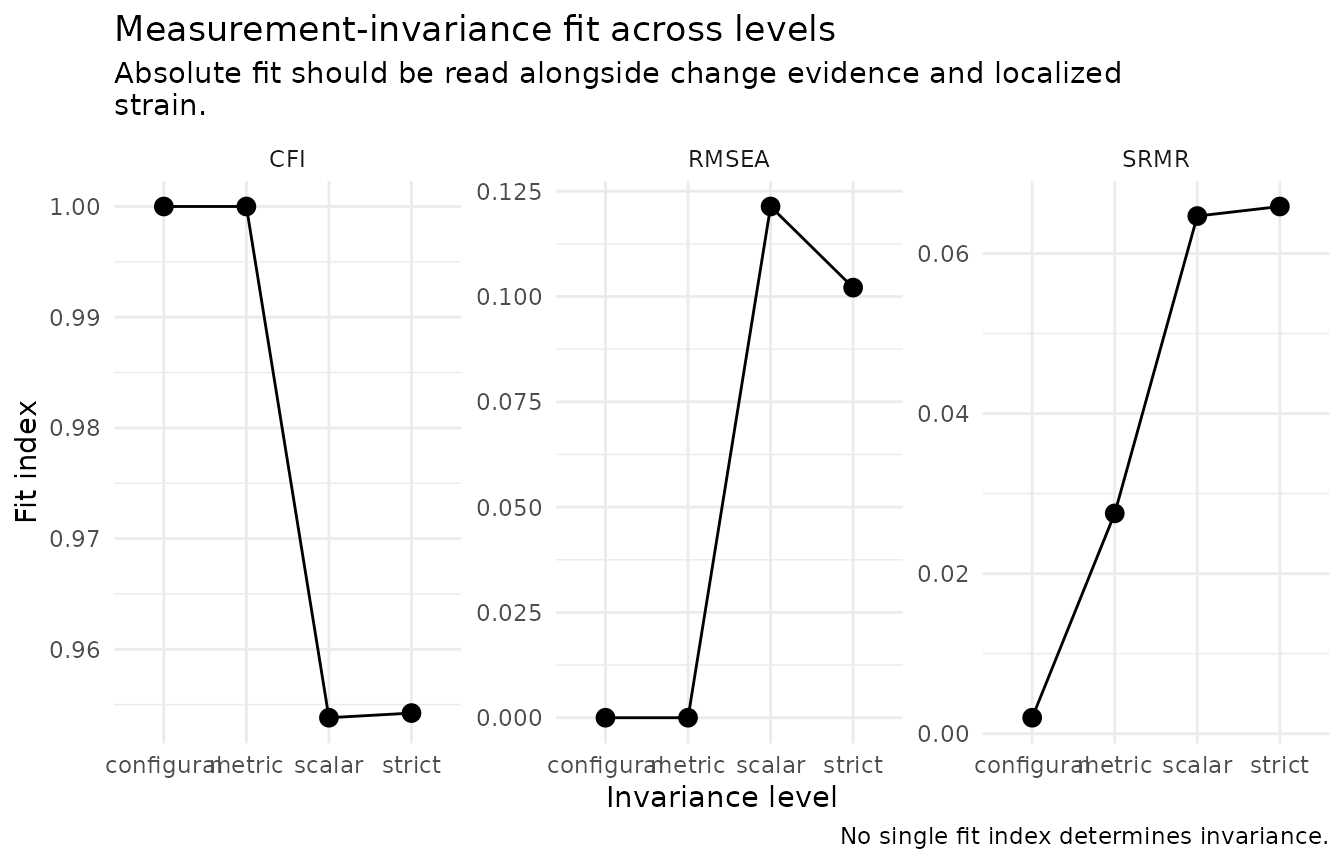

nomo_table() returns ordinary tibbles ("fit", "categories", "partial", "local_strain", "decision_log"), and plots are ordinary ggplot objects, so researchers keep direct control over reporting. The same evidence flows into nomo_report() when invariance is part of a guided workflow.

Research basis

Multiple-group factor analysis originates with Jöreskog (1971), and the configural–metric–scalar–strict hierarchy with Meredith (1993) and Vandenberg and Lance (2000). A decrease in CFI of .01 became a widely used rule after Cheung and Rensvold (2002); later work showed that sensitivity of change-in-fit indices depends on sample size and model context (Chen, 2007; Putnick & Bornstein, 2016), which is why nomologR reports several indices without a universal cutoff. Ordered-indicator sequences follow Wu and Estabrook (2016) as implemented in semTools (see also Svetina et al., 2020). Partial invariance follows Byrne, Shavelson, and Muthén (1989). Full references are in ?nomo_invariance and the research basis article.